Stochastic variational inference

\(\DeclareMathOperator*{\argmin}{arg\,min}\) \(\DeclareMathOperator*{\argmax}{arg\,max}\)

Variational inference (VI) is a framework for approximating intractable posterior distributions. In some respects, VI converts an inference problem into an optimization problem. Stochastic variational inference (SVI) is a family of methods that exploits stochastic optimization techniques to speed up variational approaches and scale them to large datasets. Here, we review SVI as introduced by Hoffman et al.

We begin by reviewing the modeling setup that Hoffman et al. focus on. Then, we describe SVI and its implementation.

The model

Although the fundamental ideas of SVI can be applied to arbitrary probabilistic models, the paper by Hoffman et al. focuses on a subset of models that are commonly used in practice. We review these modeling assumptions below.

Global and local variables

To start, we assume we have $n$ data points $\{x_1, \dots, x_n\}$ with $x_i \in \mathbb{R}^p$. The model assumes two distinct types of latent variables: local latent variables $\{z_1, \dots, z_n\}$, with $z_i \in \mathbb{R}^k$ that correspond to individual data points, and global latent variables $\beta$ that describe all of the data points. Finally, we have a set of fixed hyperparameters $\alpha$ which we assume to be constant and specified by the modeler. The joint likelihood of the model is

where we use $x$ and $z$ to denote the full data and local latent variables. For simplicity, the model assumes that only the global latent variables $\beta$ depend on the fixed hyperparameters $\alpha$. Note that the local latent variables are independent of one another.

Presented with some data, we’d like to compute the posterior distribution. In this generic model, the posterior is given by

where $z$ and $x$ are sets containing all of the local latent variables and data points in this notation. Unfortunately, the integral in the denominator is intractable for most semi-complicated models:

This intractability motivates the need for approximations to the posterior. Variational inference is a popular approach for formulating these approximations.

Example: Mixture of Gaussians

As an example of the types of models that fit into this framework, consider a simple mixture of $K$ univariate Gaussians. The model is

\begin{align} x_i | z_i = k, \mu_{z_i}, \sigma^2_0 &\sim \mathcal{N}(\mu_k, \sigma^2_0) \\ z_i &\sim \text{Categorical}(\theta), ~i=1,\dots,n \\ \mu_k &\sim \mathcal{N}(0, 1),~~~k=1,\dots,K \end{align}

where $z_i$ indicates the mixture membership of sample $i$, $\mu_k$ is the mean of mixture component $k$, $\theta \in \Delta^K$ contains the mixture probabilities, and we assume $\sigma^2_0$ is known and shared across components.

Here, the local latent variables $z$ are the sample-specific mixture memberships $\{z_i\}_{i=1}^n$, and the global latent variables $\beta$ are the mixture means $\{\mu_k\}_{k=1}^K$ and mixture probabilities $\theta$. The only hyperparameter $\alpha$ in this case is the variance $\sigma^2_0$.

Complete conditionals and the exponential family

We need one more assumption before we jump into SVI. Specifically, we assume a certain form for the complete conditional distributions. A complete conditional distribution is the distribution of a latent variable conditioned on all other latent variables and the data. In other words, it’s the posterior distribution if we also condition on all other parameters/latent variables. For example, the complete conditional for $\beta$ is $p(\beta | x, z, \alpha)$, and the complete conditional for one local variable $z_{ik}$ is $p(z_{ik} | x, \beta, z_{i, -k}, \alpha)$ where $z_{i, -k}$ contains all local latent variables for data point $i$ except the $k$th one. Recall that the local latent variables are independent of one another, so $p(z_{ik} | x, \beta, z_{i, -k}, z_{[n] \setminus i}, \alpha) = p(z_{ik} | x, \beta, z_{i, -k}, \alpha)$.

That primary assumption about the these these complete conditionals is that they’re in the exponential family. To give a brief review of the exponential family, recall that a distribution $p(x)$ with parameter vector $\theta$ belongs to the exponential family if it has the following form:

where $h(x)$ is the base measure, $\eta(\theta)$ is the natural parameter, $t(x)$ is a sufficient statistic, and $a(\theta)$ is the base measure. See the Appendix for an example of how the Gaussian its in this family. A nice/intersting property of the exponential family is that the gradient of the log-normalizer is equal to the expectation sufficient statistic:

\begin{equation} \nabla_\theta a(\theta) = \mathbb{E}[t(\theta)]. \tag{1} \label{eq:lognormalizer_identity} \end{equation}

We assume the complete conditionals $p(\beta | x, z, \alpha)$ and $p(z_{ik} | x, \beta, z_{i, -k}, \alpha)$ can be put in this exponential family form. Introducing new notation for the exponential family form of these complete conditionals, we have

\begin{align} p(\beta | x, z, \alpha) &= h(\beta) \exp\{\eta_g(x, z, \alpha)^\top t(\beta) - a_g(x, z, \alpha)\} \\ p(z_{ik} | x, \beta, z_{i, -k}, \alpha) &= h(z_{ik}) \exp\{\eta_\ell(x, \beta, z_{i, -k}, \alpha)^\top t(z_{ik}) - a_\ell(x, \beta, z_{i, -k}, \alpha)\}, \\ \end{align}

where the subscript on $\eta$ and $a$ indicates whether it corresponds to the global or local latent variables.

This exponential family assumption will simplify the downstream computation. Moreover, it’s a common assumption in many commonly-used models. Now that we’ve fully described the modeling setup, we can move onto variational inference.

Mean-field VI

As mentioned above, VI approaches seek to approximate the posterior $p(z, \beta | x, \alpha)$ with a surrogate distribution $q(z, \beta)$. One of the simplest forms of VI is mean-field VI, which assumes that the variational distribution factorizes into a product of individual variational distributions:

Mean-field assumption. \begin{equation} q(z, \beta) = q(\beta | \lambda) \prod\limits_{i=1}^n q(z_i | \phi_i), \end{equation}

where $\lambda$ and $\{\phi_i\}$ are the variational parameters that govern the global and local variational distributions, respectively.

The evidence lower bound (ELBO) is given by

\begin{equation} \mathcal{L} = \mathbb{E}_{\beta, z \sim q}\left[\log \frac{p(x, z, \beta)}{q(z, \beta)}\right] \leq \log p(x). \end{equation}

Recall that maximizing the ELBO is equivalent to minimizing the KL divergence between the true posterior and the variational posterior. We’d like to maximize the ELBO with respect to the variational parameters. We can start by maximizing with respect to the global variational parameters $\lambda$.

Rewriting the ELBO while ignoring terms that don’t depend on $\lambda$, we have

\begin{align} \mathcal{L} &= \mathbb{E}\left[\log p(x, z, \beta) - \log q(z, \beta)\right] \\ &= \mathbb{E}\left[\log p(\beta | x, z) p(x, z) - \log q(z) q(\beta)\right] & \text{(Probability chain rule)} \\ &= \mathbb{E}\left[\log p(\beta | x, z) - q(\beta)\right] + C & \text{($C$ is constant wrt $\lambda$)} \\ \end{align}

Now, taking the gradient, we have

Using our assumption that the complete conditional distributions belong to the exponential family, the gradient simplifies as follows. First, we write out the exponential family form again,

\begin{align} \nabla_\lambda \mathcal{L} &= \mathbb{E}\left[\nabla_\lambda (\log (h(\beta) \exp\{\eta_g(x, z, \alpha)^\top T(\beta) - a_g(\eta_g(x, z, \alpha))\})) \right] \\ &~~~~~- \mathbb{E}\left[\nabla_\lambda (\log (h(\beta) \exp\{\lambda^\top T(\beta) - a_g(\lambda)\})) \right]. \end{align}

Simplifying further and canceling like terms, we have

\begin{align} \nabla_\lambda \mathcal{L} &= \mathbb{E}\left[\nabla_\lambda ( \eta_g(x, z, \alpha)^\top T(\beta) - a_g(\eta_g(x, z, \alpha)) \right] \\ &-\mathbb{E}\left[\nabla_\lambda ( \lambda^\top T(\beta) - a_g(\lambda)\right]. \end{align}

Using the exponential family property described in Equation \eqref{eq:lognormalizer_identity}, we have

\begin{align} \nabla_\lambda \mathcal{L} &= \mathbb{E}\left[\nabla_\lambda ( \eta_g(x, z, \alpha)^\top \nabla_\lambda a_g(\lambda) - a_g(\eta_g(x, z, \alpha)) \right] \\ &-\mathbb{E}\left[\nabla_\lambda ( \lambda^\top \nabla_\lambda a_g(\lambda) - a_g(\lambda)\right]. \end{align}

Finally, we can compute the relevant gradients, yielding

\begin{align} \nabla_\lambda \mathcal{L} &= \mathbb{E}\left[\nabla^2_\lambda a_g(\lambda) \eta_g(x, z, \alpha) + \nabla_\lambda a_g(\lambda) + \nabla^2_\lambda a_g(\lambda) \lambda - \nabla_\lambda a_g(\lambda)\right] \\ &= \nabla^2_\lambda a_g(\lambda) (\mathbb{E}[\eta_g(x, z, \alpha)] - \lambda). \end{align}

We can see that the gradient will be zero when

Global update. \begin{equation} \lambda = \mathbb{E}[\eta_g(x, z, \alpha)]. \tag{2} \label{eq:meanvi_global_update} \end{equation}

In other words, the maximizer for the global variational parameters is the expectation of the natural parameter of the complete conditional distribution $p(\beta | x, z, \alpha)$.

A very similar derivation for the local latent variables shows that, conditioned on the global latent variables and the data, the ELBO is locally maximized when

Local update. \begin{equation} \phi_{ik} = \mathbb{E}[\eta_\ell(x, \beta, z_{i, -k}, \alpha)]. \tag{3} \label{eq:meanvi_local_update} \end{equation}

These updates for $\lambda$ and $\phi$ can be repeated in a coordinate ascent procedure, which results in a very general algorithm for mean-field VI.

Stochastic VI

We now move on to SVI aims to solve two computational issues with the coordinate ascent approach to mean-field VI.

Issue 1: Initial “garbage” updates based on random values. First, notice that prior to beginning coordinate ascent, all local and global latent variables will be initialized randomly (or possibly according to some more informed technique). If we start our ascent by first optimizing the global latent variables, the locally optimal value of $\lambda$ in Equation \eqref{eq:meanvi_global_update} will depend on the randomly-initialized values of the local latent variables $\phi$. However, these random variables won’t be informative at all, which essentially amounts to a waste of computation on the first iteration.

Issue 2: Large computational burden of iterating over complete dataset. Second, each iteration of coordinate ascent requires iterating over all of the local latent variables. For large datasets with lots of samples (many datasets now have sample sizes on the order of $10^5$ to $10^6$ or larger), this becomes computationally burdensome. Although this step can be parallelized across machines due to the independence of the local latent variables, it would be even better if we could subsample the data appropriately and not require the entire dataset.

SVI solves both of these issues with a fairly simple trick from stochastic optimization. Instead of using the entire dataset on every iteration, we can randomly sample one data point, and compute the parameter updates as if this sample were our entire dataset. In expectation, this procedure is equivalent to performing updates using the complete data.

More specifically, consider again the ELBO for our model,

We can write the ELBO separated into global and local terms:

Suppose we’re in the middle of a coordinate ascent iteration, and we’ve maximized the ELBO with respect to the local variational parameters $\phi$. Then the ELBO is a function of the global variational parameters $\lambda$, and we have

We can now make a stochastic approximation to this locally-optimized ELBO. If we randomly sample a data point index $i \sim \text{Unif}(1, n)$, we can approximate $\mathcal{L}(\lambda)$ as if this data point were the entire dataset:

Note that we’ve multipled the local term by $n$ to simulate as if we’ve replicated this data point $n$ times. We then have an unbiased estimator for the ELBO:

We can then take a stochastic, noisy gradient of this quantity, and use the Robbins Monro algorithm to optimize the ELBO.

Writing out the algorithm in steps, we have

SVI algorithm

Natural gradient

The last ingredient for SVI is the natural gradient. The natural gradient is a generalization of the generic gradient that accounts for the information geometry of a parameter space. Please see my last post for a more thorough review.

Example: Mixture of Gaussians

To show SVI in practice, we work through a simple example using a mixture of univariate Gaussians. Consider the following model:

\begin{align} x_i | z_i = k, \mu_k &\sim \mathcal{N}(\mu_k, \sigma^2_0) \
z_i &\sim \text{Multinomial}(\boldsymbol{\pi}) \
\mu_k &\sim \mathcal{N}(0, 1) \end{align}

where $\sigma^2_0$ is a known noise variance term, and $\boldsymbol{\pi} = [\pi_1, \dots, \pi_K]^\top$ is a vector of prior class probabilities. Here, we assume equal prior weight for each class, $\pi_1 = \cdots = \pi_K = \pi_0$.

Our latent variables of interest are $\{z_i\}_{i=1}^n$ and $\{\mu_k\}_{k=1}^K$. First, let’s compute the complete conditionals. For the local latent variables, we have

\begin{align} p(z_i = k | x_i, \mu_k) &= \frac{1}{C_1} p(x_i | z_i = k, \mu_k) p(z_i = k) \
&= \frac{1}{C_1} \pi_0 \mathcal{N}(x_i | \mu_k, \sigma^2_0) \end{align}

where the normalization term is a sum over mixture components,

This implies that the complete conditional is another multinomial distribution with natural parameter $\eta_{\ell}(x_i, z_{i, -k}) = \log p(z_i = k | x_i, \mu_k)$, which only depends on the global latent variables. Taking the expectation with respect to the variational distribution $q$, we have

Here, we restrict the variational variance term to be $1$ for simplicity, so this reduces to

where $\lambda_k$ is the variational mean for mixture component $k$. Note that this step effectively amounts to computing the log-likelihood of sample $i$ under each component.

Now, for the global latent variables $\mu_k$, we have the following complete conditional distribution:

\begin{align} p(\mu_k | x, z) &= \frac{1}{C_2} p(x | \mu_k, z) p(\mu_k) \
&= \frac{1}{C_2} \mathcal{N}(x | \mu_k, \sigma^2_0) \mathcal{N}(0, 1) \
&= \mathcal{N}(\widetilde{\mu}_k, \widetilde{\sigma^2}) \end{align}

where

Suppose we sample data point $x_i$ on an iteration of SVI. The locally-optimized ELBO will occur when we set the pseudo-class assignment of $x_i$ to be $k^\star = \argmax_k \phi_{ik}$. The global update will then be

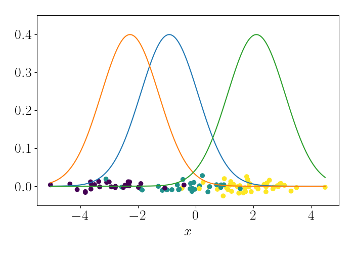
We can iteratively repeat this process, randomly sampling a data point at each iteration. To show this visually, consider the following animation. At the bottom are the data points, and the densities represent the (three) Gaussians. At each iteration, we randomly sample a point, which is shown by the red point. We then update the mean of the Gaussian that endows that point with the highest likelihood. This process is repeated.

At convergence, we have the following result.

References

• Hoffman, Matthew D., et al. “Stochastic variational inference.” Journal of Machine Learning Research 14.5 (2013).

Appendix

Gaussian in exponential family form

We can put the Gaussian in the form of the exponential family. Assume we have a dataset $x = \{x_1, \dots, x_n\}$ that is assumed to have been drawn from a Gaussian with mean $\mu$ and variance $\sigma^2$. The likelihood is then

\begin{align} p(X | \mu, \sigma^2) &= \prod\limits_{i=1}^n \frac{1}{\sqrt{2\pi \sigma}} \exp\left\{-\frac{1}{2\sigma^2} (x_i - \mu)^2\right\} \\ =& \left(\frac{1}{\sqrt{2\pi \sigma}}\right)^n \exp\left\{-\frac{1}{2\sigma^2} \sum\limits_{i=1}^n (x_i - \mu)^2\right\} \\ =& \exp\left\{\log \left((2\pi \sigma)^{-n/2}\right) - \frac{1}{2\sigma^2} \sum\limits_{i=1}^n x_i^2 + \frac{\mu}{\sigma^2} \sum\limits_{i=1}^n x_i - \frac{n}{2\sigma^2} \mu^2) \right\} \\ =& \underbrace{2\pi^{-n/2}}_{h(x)} \exp\left\{ \underbrace{\begin{bmatrix} -\frac{1}{2\sigma^2} \\ \frac{\mu}{\sigma^2} \end{bmatrix}^\top}_{\eta(\theta)} \underbrace{\begin{bmatrix} \sum\limits_{i=1}^n x_i^2 \\ \sum\limits_{i=1}^n x_i \end{bmatrix}}_{t(x)} + \underbrace{\frac{n \mu^2}{2\sigma^2} - \frac{n}{2} \log \sigma)}_{a(\theta)} \right\}. \end{align}

Monte Carlo approximation to the ELBO and its gradient

We can form an unbiased estimate of the ELBO using a naive Monte Carlo approximation. Recall that an estimator $\widehat{\theta}$ is unbiased for a quantity $\theta$ with true value $\theta^\star$ if $\mathbb{E}[\widehat{\theta}] = \theta^\star.$

Given $S$ samples from the approximate posterior, our MC estimator is

Now, we can compute the expectation of this quantity and check whether it’s equal to the true ELBO. Moving the expectation inside the sum, we have

The expectation of each term in the sum will be the same, so we can write it in terms of a generic $z$:

Thus, the expectation of our MC estimate reduces to

showing that the estimator is unbiased.

Code

import numpy as np
import matplotlib.pyplot as plt
import pandas as pd
import seaborn as sns
from scipy.stats import norm


def plot_data(means, zs, jitter=None):
	if jitter is None:
		jitter = np.random.normal(scale=0.01, size=n)

	plt.scatter(X, jitter, c=zs)
	xs = np.linspace(np.min(X), np.max(X), 1000)
	for kk in range(len(np.unique(zs))):
		ys = norm.pdf(xs, loc=means[np.unique(zs)[kk]], scale=sigma2)
		plt.plot(xs, ys)
	plt.xlabel("X")
	plt.show()

## Generate data
K = 3
mu_true = np.array([-3, 0, 2])
sigma2 = 1
n = 100
z_true = np.random.choice(np.arange(3), replace=True, size=n)
X = np.random.normal(loc=mu_true[z_true], scale=np.sqrt(sigma2))

n_iter = 5000
tau = 1
kappa = 0.9

# Initialize parameters
phi = np.random.normal(size=(n, K))
row_sums = phi.sum(axis=1)
phi = phi / row_sums[:, np.newaxis]
lam = np.random.normal(size=K)
mu_tilde = np.zeros(K)

for iter_idx in range(n_iter):

	# Randomly sample data point
	data_idx = np.random.choice(np.arange(n))
	Xi = X[data_idx]

	# Update local variables
	for k in range(K):

		# Compute log likelihood of this data point under this mixture component
		phi[data_idx, k] = norm.pdf(Xi, lam[k], sigma2)

	# Normalize
	row_sums = phi.sum(axis=1)
	phi = phi / row_sums[:, np.newaxis]

	# Update learning rate
	rho = (iter_idx + 1 + tau)**(-kappa)

	# Locally optimize
	max_idx = np.argmax(phi[data_idx, :])

	# Update global variables
	lam[max_idx] = rho * lam[k] + (1 - rho) * n / (n + 1) *  Xi

	print(lam)

plot_data(means=lam, zs=z_true)