Natural gradients

The natural gradient is a generalization of a typical gradient that accounts for the curvature of the function at hand. When applied to an optimization problem in the form of natural gradient descent, it can greatly improve the convergence speed compared to vanilla gradient descent.

Gradient descent

First, we briefly review gradient descent. Suppose we’re interested in minimizing a function $f(x) : \mathbb{R}^p \rightarrow \mathbb{R}$ with respect to $x \in \mathbb{R}^p$. Recall that the gradient $\nabla f(x)$ is the vector of partial derivatives with respect to each of its arguments:

where $x^{(i)}$ is the $i$th element of $x$.

Gradient descent is an algorithm that iteratively takes a step in the direction of the negative gradient. Let $x_t$ be the value of $x$ on the $t$th iteration. Then the gradient descent update is

where $\gamma$ is a learning rate parameter.

Steepest descent

Gradient descent is actually a special case of an algorithm known as “steepest descent.” We can think of steepest descent as a design principle for optimization algorithms: the principle says that out of all the steps we could take that have a given fixed length from $x_t$ to $x_{t+1}$, we should choose the one that reduces the cost function the most.

A key idea to notice is that how we measure the length of these steps depends on the geometry of the problem. Choosing a different measure of length will result in a different update, and a given metric could have wildly different performance for different functions.

Interestingly, gradient descent is a special case of steepest descent with one of the simplest metrics/geometries: Euclidean geometry.

To show this, consider a linear approximation of $f$ around $x_t$,

We’d like to choose an $x_{t+1}$ to minimize this. However, we need to add further constraints, since in this unconstrained problem the optimal move would be to take an infinite step in the direction of the negative gradient.

Suppose that, in addition to minimizing $f$, we simulatneously minimize one-half of the squared Euclidean distance between $x_t$ and $x_{t+1}$. That is, we choose the Euclidean distance $|x - x^\prime|$ as our distance metric. Using the linear approximation of $f$, the optimization problem then becomes

Notice that adding this term to the minimization penalizes large steps. Taking the gradient with respect to $x$ and setting it to zero, we have

Finally, we have

which corresponds to a typical gradient descent update. Notice that we can impose a learning rate $\gamma$ by penalizing a scaled Euclidean distance instead,

Thus, we can interpret gradient descent as taking a step in the direction that minimizes the function the most, but also maintains a short distance between steps. Equivalently, for a fixed step length $|x - x_t|^2_2 = c$, gradient descent steps in the direction that minimizes the function the most.

We next turn to non-Euclidean metrics.

Generalizing the metric

Notice that this choice of a Euclidean metric is a very special case, and we can generalize it further. In particular, consider an arbitrary metric $D(x, x^\prime)$ that measures a dissimilarity or distance between $x$ and $x^\prime$. Our general optimization problem is then

Amari showed that the steepest descent direction in general depends on the Riemannian metric tensor of the parameter space. Recall that the Pythagorean theorem states that for a $p$-dimensional Euclidean parameter space and two vectors $x_t$ and $x_{t+1}$, the squared length of the vector between them $dx$ is

where $dx_i$ is the $i$th element of $dx$. We can obtain a generalized version of the Pythagorean theorem for a Riemannian manifold:

If we group the scaling terms $g_{ij}$ into one $p\times p$ matrix $G$, this matrix is known as the Riemannian metric tensor.

Amari showed that the steepest descent direction in a space with metric tensor $G$ is given by

Notice that $G$ essentially acts as a “preconditioning” matrix — we premultiply the gradient by $G$ to adjust it according to the metric tensor. As a special case, we can note that this reduces to gradient descent when $G$ is the identity matrix.

Mahalanobis metric

As a first venture into non-Euclidean metrics, let’s first consider a slight generalization of the Euclidean distance: the Mahalanobis metric. This metric is given by

where $A$ is a $p \times p$ PSD matrix.

Consider the case where $A = \text{diag}(a_1, \cdots, a_p)$ is a diagonal matrix with positive diagonal elements. Notice that the resulting natural gradient will result in a simple element-wise rescaling of the gradient,

where $\rho = [1/a_1,\cdots, 1/a_p]^\top$. A trivial application of this would be a setting in which each of the elements of $x$ has a different scale (e.g., perhaps some are in miles and others are in kilometers). Using a diagonal $A$ would account for this different scales (although of course you could just rescale at the beginning).

We can again note that the Mahalanobis metric reduces to the Euclidean metric with $A$ is the identity matrix – in other words $a_1 = a_2 = \cdots = a_p = 1$.

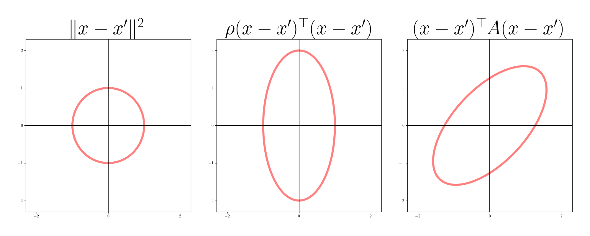
With a non-diagonal $A$, we can account for more than just orthogonal stretching of our parameter space. Heuristically, we can think of $A$ as accounting for rotations and stretching away from the Euclidean metric. Under the Euclidean metric, equidistant points form a sphere; under the Mahalanobis metric, they form an ellipsoid. The figure below shows equidistant points in two dimensions for Euclidean, diagonal Mahalanobis, and non-diagonal Mahalanobis metrics.

The gradient descent update in this case is equivalent to Newton’s method because the assumed structure of the loss function is quadratic:

As a simple example, consider the loss function

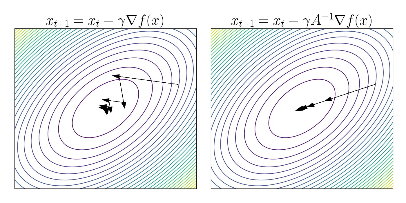
In the left figure below, we apply vanilla gradient descent under this loss function. We can see that the steps bounce around the “valley” formed by $f$.

In the right figure, we perform steepest descent using the metric $(x - x^\prime)^\top A (x - x^\prime).$ We can see that the steps go straight toward the global minimum in this case.

Fisher metric

When working with probabilistic models, we can use yet another metric that’s more friendly to probability distributions: the KL divergence. Suppose we have a likelihood model $p(x | \theta)$, where $x$ is some (fixed) data, and $\theta$ is a parameter vector. (Note that I switch notation here — what used to be $x$ is now $\theta$.)

As before, suppose $\theta_t$ is a vector of the current parameter values, and we’d like to find a new set of parameters $\theta_{t+1}$. To do so under the natural gradient framework, we solve the following problem.

Unfortunately this minimization is intractable in general. However, we can approximate the KL divergence using a second-order Taylor expansion, which turns out to be the Fisher information matrix $F$ (see Appendix for a derivation). This means that locally around $\theta_t$, we have

where

Thus, the Fisher information matrix contains all the information about the curvature in our likelihood-based loss function. Our update for the natural gradient in this setting is then

Gaussian example

Let’s consider a simple example of computing the natural gradient for a probabilistic model. Let $x \sim \mathcal{N}(\mu, \sigma^2)$, and suppose we parameterize the Gaussian in terms of its mean $\mu$ and log standard deviation $\lambda = \log \sigma$, with $\theta = (\mu, \lambda)$. The log density is

Taking the gradient, we have

\begin{align} \nabla_\theta \log p(x | \theta) &= \begin{bmatrix} \exp(-2\lambda) (x - \mu) \\ -1 + \exp(-2\lambda)(x - \mu)^2 \end{bmatrix} \\ &= \begin{bmatrix} \frac{1}{\sigma^2} (x - \mu) \\ -1 + \frac{1}{\sigma^2} (x - \mu)^2 \end{bmatrix}. \end{align}

We can then compute the Fisher information matrix as the outer product of this gradient. Plugging in the gradient for the Gaussian, we have

Expanding the outer product, we have

The off-diagonal terms will be $0$ because $\mathbb{E}[x - \mu] = \mathbb{E}[(x - \mu)^3] = 0.$ Using the definition of the variance, the top-left term will be

Finally, for the lower-right term, we can use the fact that $\mathbb{E}[(x - \mu)^3] = 3\sigma^4$, resulting in

Bringing it all together, we see that the Fisher information matrix is

Clearly, the inverse Fisher is given by

When applied as a preconditioning matrix for the gradient, this means that we’ll scale the gradient of the mean by the variance, and the scaling of the gradient of the variance will be constant.

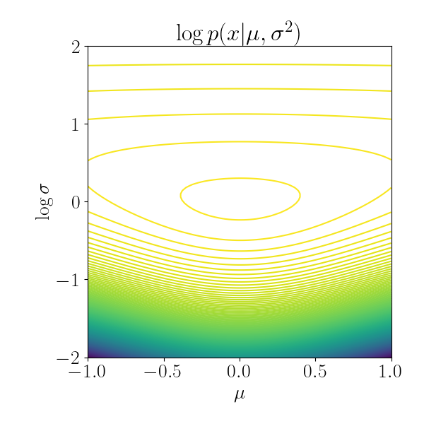
Let’s try to visualize this. I plotted the the isocontours of the univariate Gaussian below, with $\mu = 0, \log \sigma = 0$. Notice that for low values of the variance, the isocontours are much closer to each other. This implies that a gradient step in the realm of low variance will result in a much larger change in the function value compared to a step in the realm of high variance. In other words, the geometry is “steeper” with low variance.

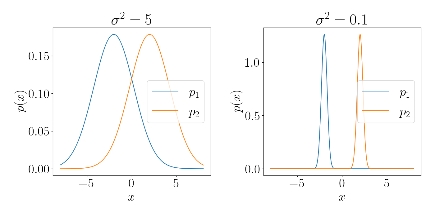
Notice that accounting for this curvature is a drastic improvement over vanilla gradient descent. To continue with the univariate Gaussian example, suppose we’re computing the distance between two Gaussians just based on their means, $\mu_1$ and $\mu_2$. Below, in each plot the means are the same, $\mu_1=-2, \mu_2=2$. However, the variances are different. Under the Euclidean metric these two pairs of Gaussians have the same distance between them. However, under the KL divergence, the Gaussians on the left are much “closer” to one another than those on the right.

Code

Code for the steepest descent example using the Mahalanobis metric:

import matplotlib.pyplot as plt
import seaborn as sns
import numpy as np
from matplotlib.patches import Ellipse
from os.path import join as pjoin
inv = np.linalg.inv
import matplotlib
font = {"size": 30}
matplotlib.rc("font", **font)
matplotlib.rcParams["text.usetex"] = True


A = np.array(
        [[1, -0.5],
        [-0.5, 1]]
)

f = lambda x1, x2: x1**2 + x2**2 - 1 * x1 * x2
fgrad = lambda x1, x2: np.array([2 * x1 - x2, 2*x2 - x1])


plt.figure(figsize=(14, 7))

plt.subplot(121)
xlimits = [-10, 10]
ylimits = [-10, 10]
numticks = 100
x = np.linspace(*xlimits, num=numticks)
y = np.linspace(*ylimits, num=numticks)
X, Y = np.meshgrid(x, y)
zs = f(np.atleast_2d(X.ravel()), np.atleast_2d(Y.ravel()))
Z = zs.reshape(X.shape)
plt.contour(X, Y, Z, levels=30)

xhat = np.array([8., 3.])

for _ in range(10):
        g = -0.5 * fgrad(*xhat)
        plt.arrow(*xhat, *g, head_width=0.5, color="black")
        xhat += g

plt.title(r"$x_{t+1} = x_t - \gamma \nabla f(x)$")
plt.xticks([])
plt.yticks([])


plt.subplot(122)
xlimits = [-10, 10]
ylimits = [-10, 10]
numticks = 100
x = np.linspace(*xlimits, num=numticks)
y = np.linspace(*ylimits, num=numticks)
X, Y = np.meshgrid(x, y)
zs = f(np.atleast_2d(X.ravel()), np.atleast_2d(Y.ravel()))
Z = zs.reshape(X.shape)
plt.contour(X, Y, Z, levels=30)

xhat = np.array([8., 3.])

for _ in range(10):
        g = -0.3 * inv(A) @ fgrad(*xhat)
        plt.arrow(*xhat, *g, head_width=0.5, color="black")
        xhat += g

plt.title(r"$x_{t+1} = x_t - \gamma A^{-1} \nabla f(x)$")
plt.xticks([])
plt.yticks([])
plt.tight_layout()
plt.show()

Code for plotting the Gaussian isocontours:

import matplotlib.pyplot as plt
import seaborn as sns
import numpy as np
from matplotlib.patches import Ellipse
from os.path import join as pjoin
from scipy.stats import norm
inv = np.linalg.inv
import matplotlib
font = {"size": 20}
matplotlib.rc("font", **font)
matplotlib.rcParams["text.usetex"] = True


mu_true = 0
sigma2_true = 1
n = 2000
data = np.random.normal(mu_true, np.sqrt(sigma2_true), size=n)

f = lambda mu, lam: n * (-0.5 * np.log(2 * np.pi) - lam) - 0.5 * np.exp(-2 * lam) * (np.sum(data**2) - 2 * mu * np.sum(data) + n * mu**2)

def fgrad(mu, lam):
        mugrad = -0.5 * np.exp(-2 * lam) * (2 * mu * np.sum(data) + n * mu)
        lamgrad = n + np.exp(-2 * lam) * (np.sum(data**2) - 2 * mu * np.sum(data) + n * mu**2)
        return np.array([mugrad, lamgrad])

plt.figure(figsize=(6, 6))
xlimits = [-1, 1]
ylimits = [-2, 2]
numticks = 100
x = np.linspace(*xlimits, num=numticks)
y = np.linspace(*ylimits, num=numticks)
X, Y = np.meshgrid(x, y)
zs = f(np.atleast_2d(X.ravel()), np.atleast_2d(Y.ravel()))
Z = zs.reshape(X.shape)
plt.contour(X, Y, Z, levels=200)
plt.tight_layout()
plt.title(r"$\log p(x | \mu, \sigma^2)$")
plt.xlabel(r"$\mu$")
plt.ylabel(r"$\log \sigma$")
plt.xticks(size=20)
plt.yticks(size=20)
plt.tight_layout()
plt.show()

References

• Amari, Shun-Ichi. “Natural gradient works efficiently in learning.” Neural computation 10.2 (1998): 251-276.
• Martens, James. “New insights and perspectives on the natural gradient method.” arXiv preprint arXiv:1412.1193 (2014).
• Ollivier, Yann, et al. “Information-geometric optimization algorithms: A unifying picture via invariance principles.” Journal of Machine Learning Research 18.18 (2017): 1-65.
• Prof. Roger Grosse’s course notes.

Appendix

Fisher information approximates the KL divergence

For notational simplicity, let $D(\theta, \theta_t) = D_{KL}(p_\theta(x) | p_{\theta_t}(x))$. Consider a second-order Taylor approximation to the KL divergence around $\theta_t$,

where $H_t$ is the Hessian of $D(\theta_t, \theta_t)$ at $\theta_t$.

The first two terms are zero. The first term is a divergence between two equal distributions, which makes the divergence zero. For the second term, we can see that

\begin{align} \nabla_\theta D(\theta, \theta_t) &= \nabla_\theta \mathbb{E}_{p(x | \theta)}\left[\log \frac{p(x | \theta)}{p(x | \theta_t)}\right] \\ &= \mathbb{E}_{p(x | \theta)}\left[\nabla_\theta \log \frac{p(x | \theta)}{p(x | \theta_t)}\right] & \text{(Swap $\nabla$ and $\mathbb{E}$)} \\ &= \mathbb{E}_{p(x | \theta)}\left[\nabla_\theta \log p(x | \theta)\right] & \text{(Grad. doesn’t depend on $\theta_t$)} \\ &= 0. \end{align}

The final line comes from the fact that the expectation of the score is always $0$.