Andy Jones
Statistical whitening transformations
Statistical “whitening” is a family of procedures for standardizing and decorrelating a set of variables. Here, we’ll review this concept in a general sense, and see two specific examples.
Introduction
Suppose data matrix $X \in \mathbb{R}^{n \times p}$ (where each row is a sample) has covariance matrix $\Sigma = \frac1n X^\top X$. A whitening transformation is one that transforms the data such that the transformed data’s covariance is the identity matrix $I_p$.
In particular, the $p \times p$ whitening matrix $W$ satisfies
\[\frac1n W^\top X^\top X W = W^\top \Sigma W = I_p.\]For this to be the case, $W$ must satisfy
\[W W^\top = \Sigma^{-1}.\]We can whiten the data as $Y = XW$, where again $\frac1n Y^\top Y = I_p$.
However, the constraint above that $W W^\top = \Sigma^{-1}$ does not uniquely pin down a way to find $W$ when presented with data $X$. Various statistical whitening procedures have been proposed, and the central choice in all of these is how to compute $W$.
To see that $W$ is not unique, consider that taking the square root of $W W^\top$ yields
\[W = \Sigma^{-1/2}.\]However, this solution for the square root is actually incomplete. In fact, there are many solutions:
\[W = Q\Sigma^{-1/2}\]where $Q$ is an arbitrary orthonormal matrix ($Q^\top Q = I$). In other words, we can arbitrarily rotate $W$ and still satisfy these conditions. To see this note that
\begin{align} W W^\top &= Q \Sigma^{-1/2} (Q \Sigma^{-1/2})^\top \\ &= Q \Sigma^{-1/2} \Sigma^{-1/2} Q^\top \\ &= \Sigma^{-1}. \end{align}
Thus, any choice of an orthonormal matrix $Q$ satisfies our original constraint. So deciding on a value of $W$ actually boils down to deciding on a value for $Q$.
To dive more deeply, consider the eigendecomposition of $\Sigma$:
\[\Sigma = U \Lambda U^\top\]where the columns of $U$ are $\Sigma$’s eigenvectors, and $\Lambda$ is a diagonal matrix containing $\Sigma$’s eigenvalues. Its inverse square root is then
\[\Sigma^{-1/2} = U \Lambda^{-1/2} U^\top.\]This implies that
\[W = Q U \Lambda^{-1/2} U^\top.\]Thus, the final whitening procedure can be written as
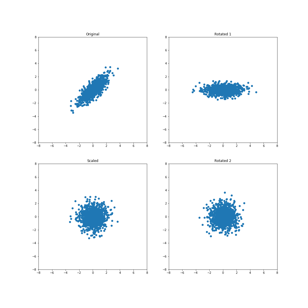
\[XW = X Q U \Lambda^{-1/2} U^\top.\]Notice that $U^\top$ rotates the data to align with the eigenbasis, $\Lambda^{-1/2}$ scales the data so that each dimension has the same variance, and $QU$ rotates the data again.
The transformation $X \Lambda^{-1/2} U^\top$ already “whitens” the data, so the final rotation by $QU$ is what distinguishes whitening procedures.
Here, we’ll discuss two of the simplest whitening procedures: ZCA whitening and PCA whitening.
ZCA whitening
Even though whitening standardizes the variance of each dimension, one may still desire that the whitened data is correlated with the original data in each dimension. This is was ZCA-based whitening seeks to achieve. ZCA stands for zero-phase component analysis.
ZCA whitening seeks to find a transformation $W$ such that the distance between the original data $X$ and the whitened data $Y = XW$ is minimized. Consider a data vector $x \in \mathbb{R}^p$ and its whitened counterpart $y \in \mathbb{R}^d$. ZCA whitening seeks to minimize
\begin{align} (y - x)^\top (y - x) &= \text{tr}(y^\top y) - 2 \text{tr}(yx^\top) + \text {tr}(x^\top x) \\ &= \text{tr}(I_p) - 2 \text{tr}(xy^\top) + \text{tr}(x^\top x) \\ \end{align}
Since $\text{tr}(x^\top x)$ and $\text{tr}(I_p)$ don’t depend on $W$, minimizing the expression above is equivalent to maximizing
\[\text{tr}(xy^\top) = \sum\limits_{j = 1}^p x_{(j)}^\top y_{(j)} = \sum\limits_{j = 1}^p \text{cov}(x_{(j)}, y_{(j)})\]where $x_{(j)}$ and $y_{(j)}$ are the $j$th features of the data and the whitened data, respectively.
Recalling that $W = Q\Sigma^{-1/2}$, we have that
\[\text{tr}(x^\top y) = \text{tr}(x^\top x W) = \text{tr}(\Sigma Q \Sigma^{-1/2}) = \text{tr}(Q \Sigma^{1/2}).\]It turns out (see Proposition 1 in Kessy et al. for a simple proof) that this is maximized when $Q$ is the identity matrix $I_p$. This means that the whitening transformation is simply the inverses square root of the covariance matrix:
\[W = \Sigma^{-1/2}.\]Putting this all together, the transformation is
\begin{align} XW &= X Q\Sigma^{-1/2} \\ &= X I_p \Sigma^{-1/2} \\ &= X \Sigma^{-1/2}. \end{align}
As we can see, ZCA whitening is essentially just decorrelating the variables, and scaling each by its inverse standard deviation.
The series of transformations can be seen in the figure below:
PCA whitening
PCA (principal component analysis) whitening has a similar flavor to ZCA whitening, but its objective is slightly different. Rather than maximizing the cross-covariance between $X$ and $Y$ in each dimension separately, PCA whitening attempts to maximize the cross-covariance of each whitened dimension with all of the original dimensions.
In particular, for a whitened variable $y_{(i)}$, PCA whitening seeks to maximize $\sum\limits_{j = 1}^p \text{cov}(y_{(i)}, x_{(j)})^2$.
Across variables, this is equivalent to maximizing
\begin{align} \text{tr}(x^\top y y^\top x) &= \text{tr}(x^\top xW W^\top x^\top x) \\ &= \text{tr}(\Sigma W W^\top \Sigma) \\ &= \text{tr}(\Sigma Q \Sigma^{-1/2} \Sigma^{-1/2} Q^\top \Sigma) \\ &= \text{tr}(Q \Sigma Q^\top). \end{align}
It turns out (again, see Proposition 1 in Kessy et al. for a proof) that this is maximized when we let the columns of $Q$ be the eigenvectors of $\Sigma$. Thus, PCA whitening rotates the standardized variables back into the original basis.
References
- Kessy, Agnan, Alex Lewin, and Korbinian Strimmer. “Optimal whitening and decorrelation.” The American Statistician 72.4 (2018): 309-314.
- Joe Marino’s blog post on statistical whitening.
- PCA whitening tutorial from Stanford.
Acknowledgements
- Thanks to Brett Jurman for noticing errors with matrix dimensions.