Andy Jones
Introduction to VC dimension
VC dimension is a measure of the complexity of a statistical model. In essence, a model with a higher VC dimension is able to learn more complex mappings between data and labels. In this post, we’ll firm up this definition and walk through a couple simple examples.
Basic learning setup
Before we jump into the definition, let’s set up a generic learning situation. Consider the case of binary classification: we are given some data $\mathcal{X} \in \mathbb{R}^d$ and labels $\mathcal{Y} \in \{0, 1\}$, which come from some joint distribution $\mathcal{D}$. Our goal in this setting is to find a function $h : \mathcal{X} \mapsto \mathcal{Y}$ that minimizes the empirical risk (classification error).
When searching for the best function, we often restrict ourselves to a subset of all possible functions. We call this set the “hypothesis class”, denoted $\mathcal{H}$, where each element is a hypothesis mapping data to labels.
As a trivial example, consider the case where $\mathcal{X} \in \mathbb{R}$, and $\mathcal{H}$ is a set containing two constant hypotheses: one that predicts the label $1$ always, and another that predicts $0$ always. Clearly, this type of hypothesis class will be useless in most situations.
As a slightly more expressive example, consider the case where $\mathcal{X} \in \mathbb{R}$, and $\mathcal{H}$ is the set of all threshold functions, i.e., $\mathcal{H} = { h_a : a \in \mathbb{R} }$ where $h_a$ classifies a data point based on whether it’s less that $a$; that is, $h_a(x) = \mathbb{1}_{x < a}$. This class at least gives us some ability to discriminate between points, but it’s still fairly limited in the types of data that it could perform well on.
Shattering
Some hypothesis classes are more expressive than others. One way to measure the “expressiveness” of a hypothesis class is to directly count the number of functions that it can represent. This leads us to the idea of shattering.
Consider again the binary classification setup, in which we’re given some data from the domain $\mathcal{X}$, and we’d like to predict $0$ or $1$ for each data point. Specifically, consider a sample $\mathcal{C} \subset \mathcal{X}$ containing $n$ data points. Because $n$ is finite, there are only a finite number of ways to possibly label the data; specifically, there are $2^n$ labelings (each data point could be given a $0$ or $1$).
Now, we say that a hypothesis class $\mathcal{H}$ shatters $\mathcal{C}$ if it’s able to represent all $2^n$ of these functions. Said another way, if we’re given any possible labeling of $\mathcal{C}$, by using hypotheses within $\mathcal{H}$ we will always be able to find a hypothesis that achieves zero error.
To build some intuition, let’s look at our simple examples from above again and see which types of data they can shatter.
Constant classifiers
Let’s examine the case where our hypothesis class is the set of two hypotheses where one always predicts $1$, and the other always predicts $0$. Let’s say we observe a sample $C \subset X$ that contains exactly one data point (it’s on the real line, so it’s just a scalar value). In this case, the dataset could have $2^1 = 2$ possible labelings – that is, the point could either be labeled $0$ or $1$. Our set of constant classifiers could correctly handle either of these labelings, and so it shatters this set of data.
Now consider the case where our data sample has two points. There are $2^2 = 4$ possible labelings here ($\{0, 0\}, \{1, 0\}, \{0, 1\},$ and $\{1, 1\}$). The constant classifiers would be able to correctly label the situations where the labels are $\{0, 0\}$ or $\{1, 1\}$, but not $\{1, 0\}$ or $\{0, 1\}$. Thus, it doesn’t shatter a sample with two points.
Threshold classifiers
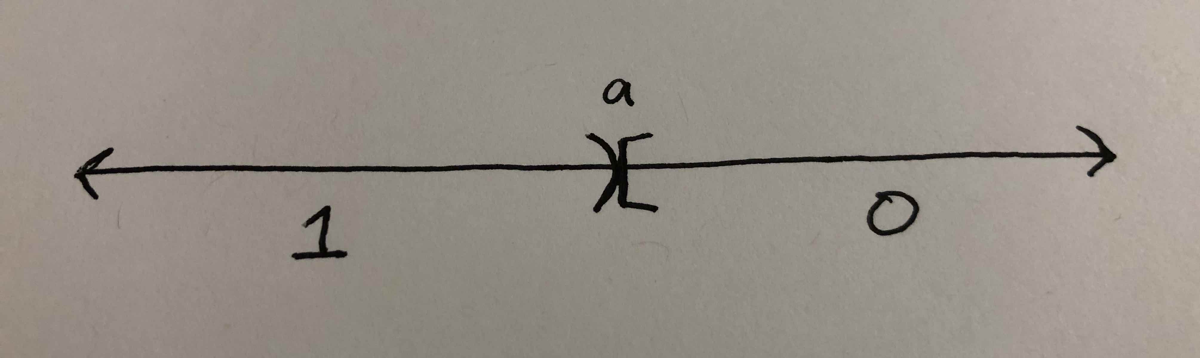
Let’s look at our class of threshold classifiers: $\mathcal{H} = { h_a : a \in \mathbb{R} }$, $h_a(x) = \mathbb{1}_{x < a}$. An example is depicted visually here, showing that points on the real line less than $a$ are classified as $1$, and points greater than $a$ are classified as $0$.
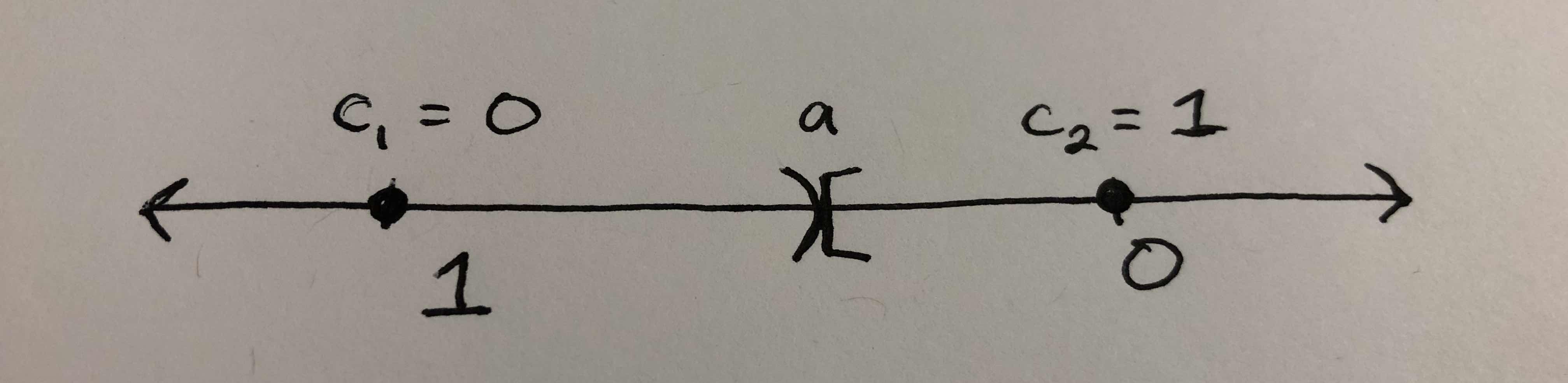
It clearly shatters $\mathcal{C}$ the case with just one data point. In the case with two data points, it actually fails to shatter $\mathcal{C}$. Let’s say the two points are $c_1$ and $c_2$, where $c_1 < c_2$. If the label of $c_1$ is $1$ and the $c_2$’s label is 0, then the hypothesis class can correctly label the points. But if the respective labeling is $0$ and $1$, it cannot, because each hypothesis can only assign the label $1$ to the lesser of two points. For a visual explanation, consider the picture below. No matter where we slide the parameter $a$ along the real line, we’ll never be able to classify $c_1$ and $c_2$
Interval classifiers
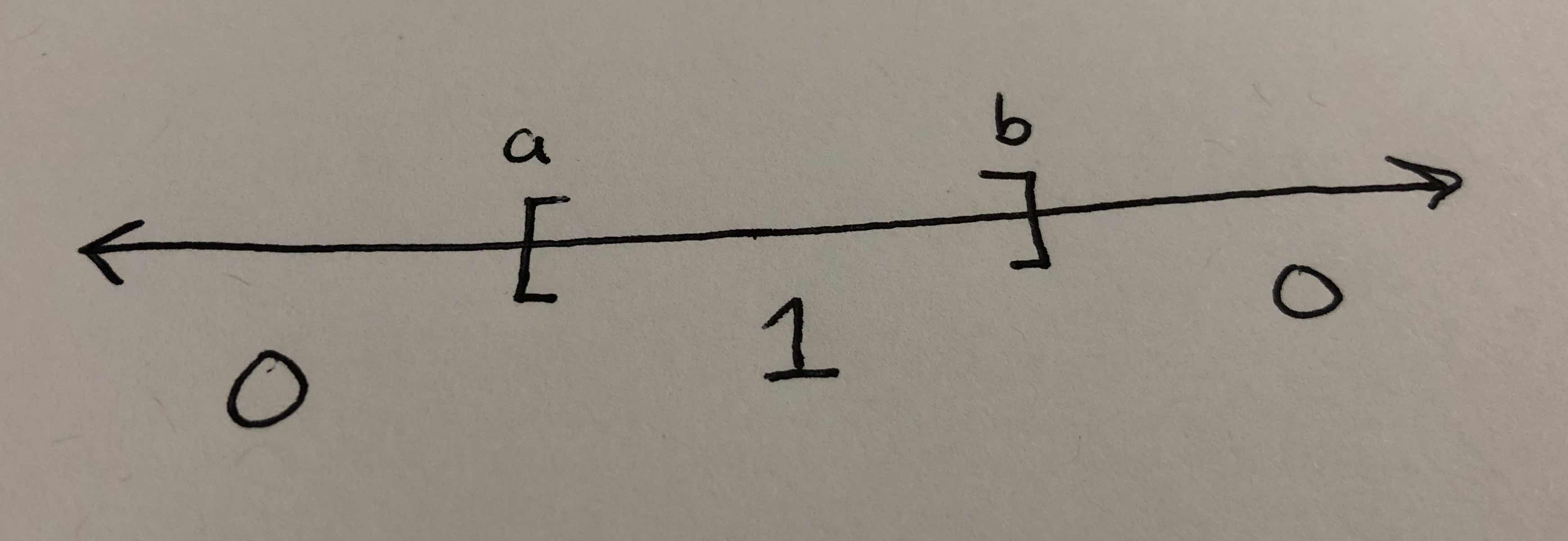
To see an example that shatters a dataset of size greater than one, consider the class of interval classifiers, $\mathcal{H} = { h_{a, b} : a, b \in \mathbb{R}, a < b }$ where $h_{a, b}(x) = \mathbb{1}_{[x \in (a, b)]}$. Depicted visually here:
The class trivially shatters the case with one point.
This class also shatters $\mathcal{C}$ when it contains two points – it can always just wrap the interval around the point(s) that are labeled $1$.
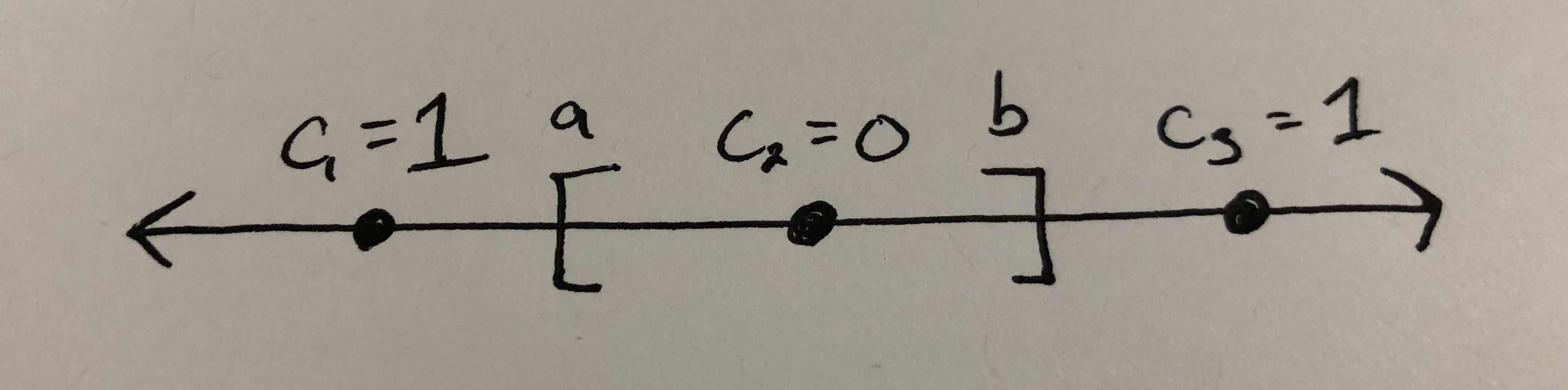
Does it shatter a set with three points? Consider three points $c_1$, $c_2$, $c_3$, where $c_1 \leq c_2 \leq c_3$. If these points are labeled $1$, $0$, $1$, respectively, the interval classifiers can never properly label the points. Consider the picture below – we’ll never be able to slide $a$ and $b$ such that only $c_1$ falls within $[a, b]$.
VC dimension
After all that setup, we’re finally ready to define VC dimension (and it will be simple now that we have the background).
The VC dimension of a hypothesis class $\mathcal{H}$ is the size of the largest set $\mathcal{C}$ that $\mathcal{H}$ is able to shatter.
In our examples:
- The VC dimension of constant classifiers is 1.
- The VC dimension of threshold classifiers is 1.
- The VC dimension of interval classifiers is 2.
Note that we have only considered extremely simple examples here (one-dimensional data with discrete labels). In practice computing the VC dimension will be more complex (think about the expressiveness of neural networks, for example).
It’s also possible for the VC dimension to be infinite. In fact, if this is the case, then it turns out that $\mathcal{H}$ is not PAC learnable. This should intuitively make sense, because an infinite VC dimension implies that it will be very difficult to search over the set of hypotheses, and the class is so expressive that it’s basically meaningless.
References
- Shai Shalev-Shwartz and Shai Ben-David. 2014. Understanding Machine Learning: From Theory to Algorithms. Cambridge University Press, New York, NY, USA.