Variational inference for Gaussian processes

\(\DeclareMathOperator*{\argmin}{arg\,min}\) \(\DeclareMathOperator*{\argmax}{arg\,max}\)

Gaussian processes (GPs) can be used as flexible priors for functions in a range of problem types, from regression to dimensionality reduction. Performing inference and prediction with GPs, however, can be computationally demanding, so many approximation methods have been developed. Here, we review a method that formalizes a popular approximation tool for GPs — inducing points — in the context of variational inference.

We first provide a basic review of GPs and GP regression, and then we describe the variational approximation.

Gaussian process review

Recall that a GP is a collection of random variables, any finite subset of which follows a multivariate normal distribution. In the regression setting, we can think of a GP as a prior over functions mapping from inputs to outputs.

To be more concrete, let $y \in \mathbb{R}^n$ be a vector of response variables, and let $X$ be an $n \times p$ matrix of covariates. We can describe the model for GP regression in at least three distinct ways. We outline these three below.

Model formulation 1

The first model for GP regression describes a GP explicitly as a prior for the regression function $f : \mathbb{R}^p \rightarrow \mathbb{R}$, which maps from inputs to outputs. The model takes the following form:

\begin{align} y_i &= f(x_i) + \epsilon \\ f &\sim \mathcal{GP}(\mu(X), K(X, X)) \\ \epsilon &\sim \mathcal{N}(0, \sigma^2 I_n). \end{align}

In this model, the function $f$ is a draw from a GP prior, which is parameterized by a mean $\mu$ and covariance function $K$.

Model formulation 2

A second, equivalent way to describe this model is by representing the response variables as a draw from a multivariate normal distribution,

Model formulation 3

The final equivalent way to describe a GP regression model is to include the (unobserved) function evaluations $f_n = \{f(x_i)\}_{i=1}^n$. To do this, we notice that our observations $y$ are noise-corrupted versions of these function evaluations. Denoting the underlying function evaluations as $f_n$, we can then write the joint model as

In this notation, our noise model is $p(Y | f_n) = \mathcal{N}(Y | f_n, \sigma^2 I_n)$, and our GP model is $p(f_n | X) = \mathcal{N}(f_n | \mu(X), K(X, X))$.

Posterior predictive

Under any of these models, using properties of the multivariate normal, we can easily compute the posterior predictive distribution for a set of new test input points $X^\star$:

\begin{equation} p(Y^\star | X^\star, X, Y) = \mathcal{N}(Y^\star | K_{X^\star X} K_{XX}^{-1} Y, K_{X^\star X^\star} - K_{X^\star X} K_{XX}^{-1} K_{X^\star X}) \tag{1} \label{eq:posteriorpredictive} \end{equation}

where $K_{AB}$ denotes the matrix of kernel evalations for all pairwise combinations of the rows of $A$ and $B$.

Having reviewed GP regression, we’ll now provide some background on inducing points, which will be the main building block for the variational approximation.

Inducing points

Computing the covariance of the posterior predictive in Equation \eqref{eq:posteriorpredictive} is computationally demanding due to the need to invert the $n \times n$ matrix $K_{XX}$. Without any further optimization, this will cost $\mathcal{O}(n^3)$. Thus, it’s useful to have good approximations to the posterior predictive that aren’t so expensive. One popular family of approximations involves using “inducing points”.

To give a big of background on inducing points, consider the setting of GP regression again, using the same notation as the first section. In addition to our outputs $y$ and our inputs $X$, we create $m$ “inducing locations” $\bar{X} = [\bar{x}_1^\top \cdots \bar{x}_m^\top]^\top,$ each of which has an associated “pseudo observation” $\bar{f} = [\bar{f}_1, \dots, \bar{f}_m]^\top$. We typically assume that there are fewer inducing points than data points, $m < n$. The reason for this is to gain computational savings, as we will see in a moment. We can choose the inducing locations, but the pseudo observations aren’t observed. Our joint model is then

Placing a Gaussian prior on the psuedo observations $\bar{f} \sim \mathcal{N}(0, K(\bar{X}, \bar{X}))$, we can analytically compute the posterior $p(\bar{f} | Y, X, \bar{X})$. Given a set of test points $X^\star$, we can also analytically compute the posterior predictive

\begin{align} p(Y^\star | X^\star, Y) &= \int p(Y^\star, f, \bar{f} | X^\star, Y) d \bar{f} \\ &= \int p(Y^\star | f, \bar{f}, X^\star, Y) p(f | \bar{f}) p(\bar{f}) d \bar{f} \end{align}

where we have stopped explicitly conditioned on $X$ and $\bar{X}$ for simplicity.

The advantage of this approach is that it’s less computationally demanding than computing the true posterior predictive. Here, the computational cost is reduced to $\mathcal{O}(n^2 m)$. Recall that we typically assume $m < n$, so this is faster than inverting the original matrix.

This approach was first proposed by Snelson and Ghahramani, where it was called the sparse pseudo-input Gaussian process (SPGP).

In this paper, the authors showed we can compute the log marginal likelihood as

\begin{align} p(y | X, \bar{X}, \theta) &= \int p(y | X, \bar{X}, \bar{f}) p(\bar{f} | \bar{X}) d\bar{f} \\ &= \mathcal{N}(y | 0, K_{X \bar{X}} K_{\bar{X} \bar{X}}^{-1} K_{\bar{X} X} + \Lambda + \sigma^2 I_n). \end{align}

Furthermore, we can optimize this likelihood with respec to the inducing locations $\bar{X}$. We demonstrate this approach in a simple example in the example section below.

Variational inference

Suppose we’re interested in computing the posterior $p(f, \bar{f} | Y)$. Recall that this factorizes under the model as

This is due to the assumption that $f$ and $y$ are conditionall independent given $\bar{f}$.

We can compute $p(f | \bar{f})$ in closed form, but $p(\bar{f} | y)$ is intractable. We can thus take a variational inference approach, and approximate this posterior. In particular, assume we approximate it as

Thus, $\phi$ is our free variational distribution. Following a typical variational inference approach, we can minimize the KL divergence between these two distributions, which is equivalent to maximizing the evidence lower bound (ELBO):

We can simplify the ELBO as follows using the factorization of the joint model and variational distribution:

\begin{align} \mathbb{E}_q \left[ \log \frac{p(Y, f, \bar{f})}{q(f, \bar{f})} \right] &= \mathbb{E}_q \left[ \log \frac{p(Y | f) p(f | \bar{f})}{p(f | \bar{f}) \phi(\bar{f})} \right] \\ &= \mathbb{E}_q \left[ \log \frac{p(Y | f)}{\phi(\bar{f})} \right]. \end{align}

We can then maximize this bound with respect to $\phi$. In this case, we get closed form solution for the optimal $\phi$ for a given set of inducing locations $\bar{X}$. The ELBO $\mathcal{L}$, which in this case is a function of the inducing locations $\bar{X}$, is then

\begin{equation} \mathcal{L}(\bar{X}) = \log [\mathcal{N}(Y | 0, Q_{nn} + \sigma^2 I)] - \frac{1}{2\sigma^2} tr(\widetilde{K}) \tag{2} \label{eq:bayesianlikelihood} \end{equation}

where $Q_{nn} = K_{nm} K_{mm}^{-1} K_{mn}$ and $\widetilde{K} = K_{nn} - K_{nm}K_{mm}^{-1} K_{mn}$.

As in the SPGP model, we can then maximize this ELBO with respect to the inducing locations $\bar{X}$ (as well as kernel hyperparameters) using gradient-based methods.

The key term in Equation \eqref{eq:bayesianlikelihood} that distinguishes this variational approach from the SPGP model is $\widetilde{K}$. This term effectively serves as a regularization, which can help to prevent overfitting of the inducing points, as well as the kernel hyperparameters and the noise variance $\sigma^2$.

Example

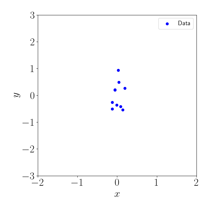
Consider the following example. Suppose we have a set of $n=10$ training points, all of whose $x$ values are centered around $0$. Given that the points are so tightly clustered together, we don’t necessarily need to compute the full covariance among all of them. Instead, we can leverage an inducing point approximation to model the region that contains the data.

Here’s a plot of our data:

Sparse pseudo inputs GP (SPGP)

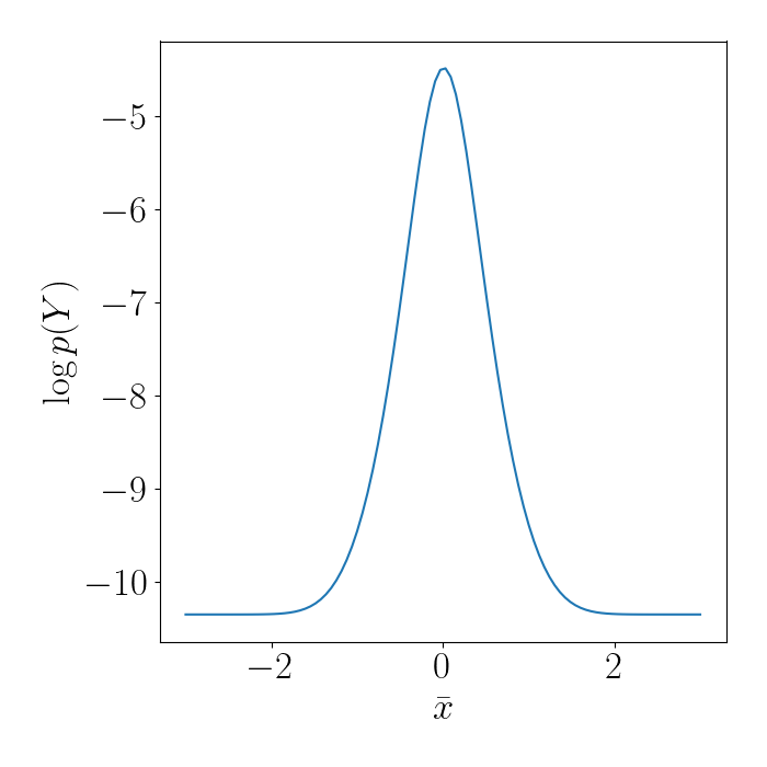
Suppose we use $m=1$ inducing point, $\bar{x}$. We can compute the log marginal likelihood of the data under various settings of $\bar{x}$. Shown below, we can see that it clearly reaches a maximum around $\bar{x} = 0$, which is where the data is dense.

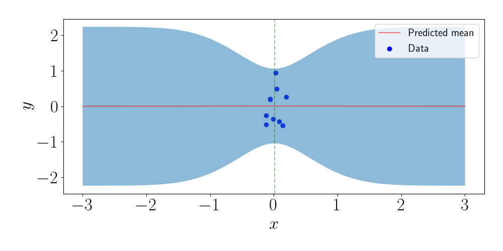
We can then make predictions for unseen points. Notice below that, although we only used one inducing point, our model is still able to fit the data very well because it’s clustered so closely together.

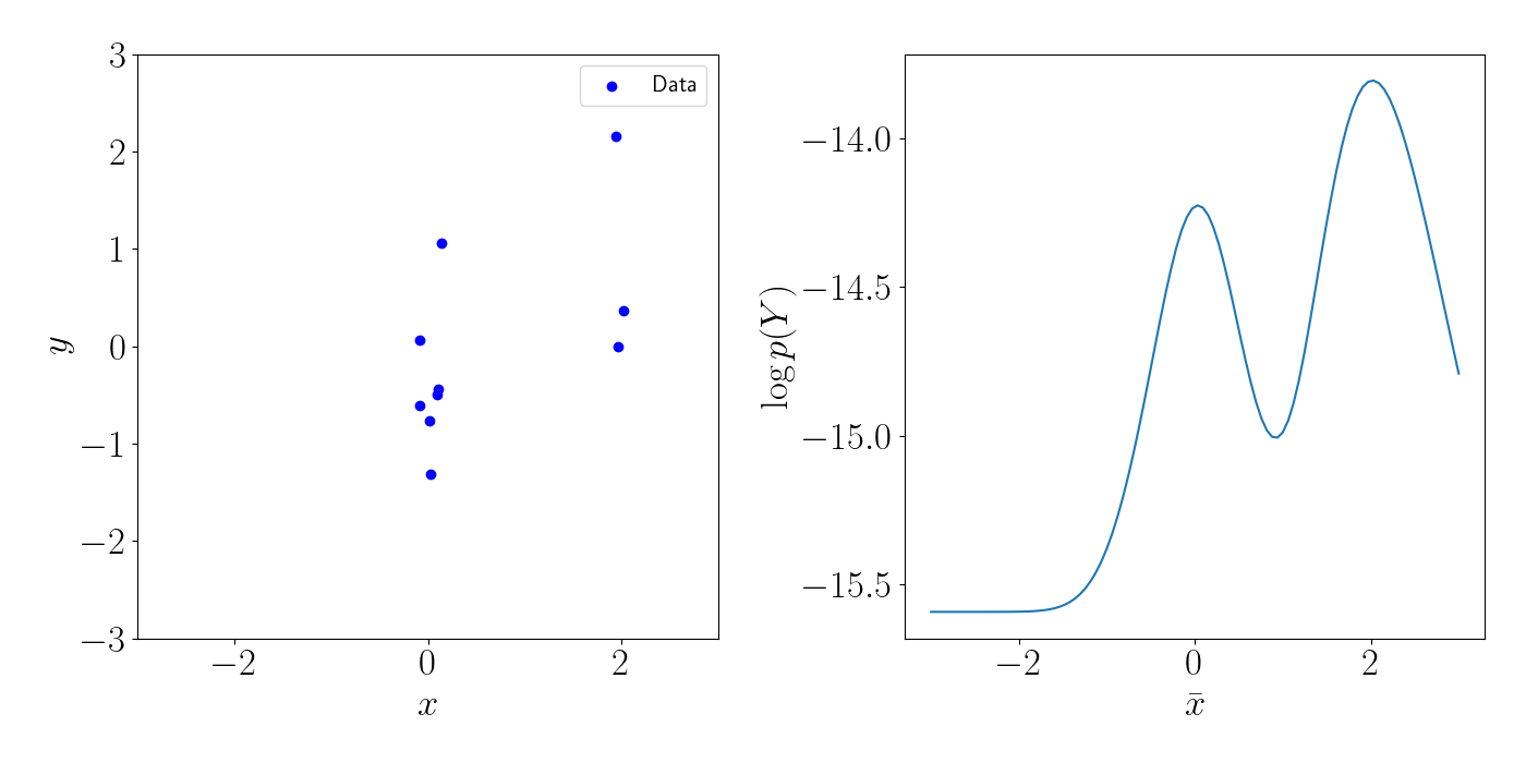
Note that in general, the marginal likelihood will not be this well-behaved. For example, consider a slight deviation from the above example, where we instead have two clusters of points, shown in the left plot below. In this case, there will be two (local) maxima for the inducing points, each centered on the location of the clusters. This is shown in the right plot below.

Bayesian approach

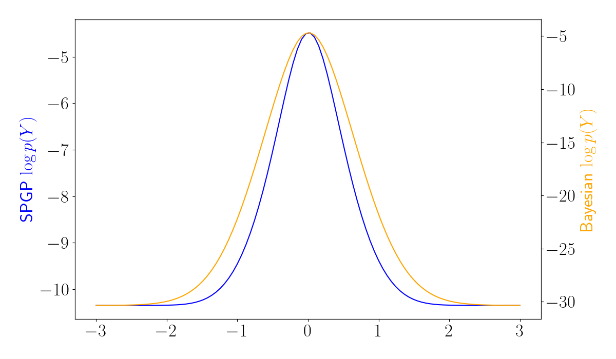
Let’s now compare the SPGP results to the Bayesian approach presented above. Below, we use the same unimodal data, and we plot the log marginal likelihood for each approach. We can see that the Bayesian model (orange) regularizes the loss surface.

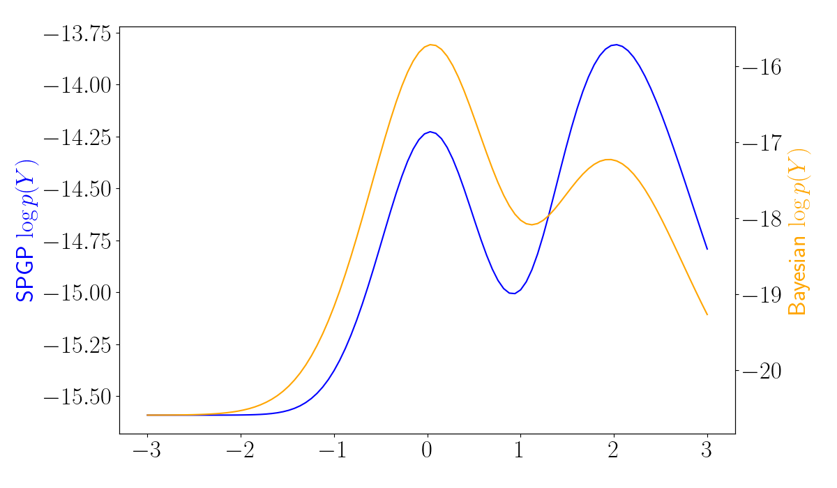
The difference between the SPGP and variational approaches becomes even more evident in the bimodal data setting. Below, we plot the log marginal likelihoods for the SPGP and Bayesian models. We can see that the Bayesian model has a higher likelihood when the inducing point is placed in the location with the highest data density (around 0). In contrast, SPGP is prone to “overfit” the data, and can instead encourage the inducing point to center around outliers.

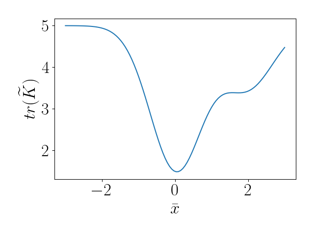
To look at this more closely, we can examine the value of the regularization term $\widetilde{K}$. Below, we see that the regularization term encourages the inducing point to center around the data-dense regions, as expected.

Conclusion

In this post, we examined an approach that uses variational inference to form an inducing point approximation for GP regression. This variational approach both formalizes our framing of inducing points using existing ideas from variational inference, and it also serves as a principled regularization approach. Leveraging variational inference for inducing point methods has now become widely popular, and it has been extended to the latent variable modeling setting, among others.

References

• Titsias, Michalis. “Variational learning of inducing variables in sparse Gaussian processes.” Artificial intelligence and statistics. PMLR, 2009.
• Snelson, Edward, and Zoubin Ghahramani. “Sparse Gaussian processes using pseudo-inputs.” Advances in neural information processing systems 18 (2005): 1257-1264.
• Titsias, Michalis, and Neil D. Lawrence. “Bayesian Gaussian process latent variable model.” Proceedings of the Thirteenth International Conference on Artificial Intelligence and Statistics. JMLR Workshop and Conference Proceedings, 2010.

Code

Below is the code for the unimodal example shown above.

import numpy as np
import autograd.numpy as np
import autograd.scipy.stats.multivariate_normal as mvn
import matplotlib.pyplot as plt
import seaborn as sns
from scipy.stats import multivariate_normal as mvnpy
import matplotlib
from autograd import grad, value_and_grad
from scipy.optimize import minimize
inv = np.linalg.inv

font = {"size": 25}
matplotlib.rc("font", **font)
matplotlib.rcParams["text.usetex"] = True

def unpack_params(params):
	return np.reshape(params, (m, 1)), None

def rbf_covariance(x, xp):
	output_scale = 1
	lengthscales = 1
	diffs = np.expand_dims(x / lengthscales, 1)\
		  - np.expand_dims(xp / lengthscales, 0)
	return output_scale * np.exp(-0.5 * np.sum(diffs**2, axis=2))

def gaussian_logpdf(x, mean, cov):
	p = x.shape[0]
	return -0.5 * (p * np.log(2. * np.pi) + np.linalg.slogdet(cov)[1] + (x - mean).T @ inv(cov) @ (x - mean))

def neg_log_marginal_likelihood(params):

	Xbar, kernel_params = unpack_params(params)

	Kxbarxbar = k(Xbar, Xbar)
	Kxbarx = k(Xbar, x)
	Kxbarxbar_inv = inv(Kxbarxbar)
	cross_prod_mat = Kxbarx.T @ Kxbarxbar_inv @ Kxbarx
	
	Q = np.diag(np.diag(Kxx - cross_prod_mat)) + cross_prod_mat
	marginal_cov = Q + sigma2 * np.eye(n)
	LL = mvn.logpdf(x.squeeze(), np.zeros(n), marginal_cov)

	return -LL

def bayesian_neg_log_marginal_likelihood(params):

	Xbar, kernel_params = unpack_params(params)

	Kxbarxbar = k(Xbar, Xbar)
	Kxbarx = k(Xbar, x)
	Kxbarxbar_inv = inv(Kxbarxbar)
	cross_prod_mat = Kxbarx.T @ Kxbarxbar_inv @ Kxbarx

	regularization_term = 0.5 * (1 / sigma2) * np.trace(Kxx - cross_prod_mat)
	
	Q = np.diag(np.diag(Kxx - cross_prod_mat)) + cross_prod_mat
	marginal_cov = Q + sigma2 * np.eye(n)
	LL = mvn.logpdf(x.squeeze(), np.zeros(n), marginal_cov) - regularization_term

	return -LL

if __name__ == "__main__":

	# Set up kernel
	k = rbf_covariance

	# Draw samples from GP
	n = 10
	sigma2 = .25
	x = np.random.normal(loc=0, scale=0.1, size=n)
	x = np.expand_dims(x, axis=1)
	Kxx = k(x, x)

	y = mvnpy.rvs(mean=np.zeros(n), cov=Kxx + sigma2 * np.eye(n))

	y -= np.mean(y)

	plt.figure(figsize=(7, 7))
	plt.scatter(x, y, c="blue", label="Data")
	plt.xlabel(r"$x$")
	plt.ylabel(r"$y$")
	plt.xlim([-2, 2])
	plt.ylim([-3, 3])
	plt.legend(prop={'size': 15})
	plt.tight_layout()
	plt.show()

	# Get predictions from GP
	n_test = 100
	xstar = np.linspace(-3, 3, n_test)
	xstar = np.expand_dims(xstar, 1)
	Kxstarx = k(xstar, x)
	Kxstarxstar = k(xstar, xstar)
	ystar_mean = Kxstarx @ inv(Kxx + sigma2 * np.eye(n)) @ y
	ystar_cov = Kxstarxstar - Kxstarx @ inv(Kxx + sigma2 * np.eye(n)) @ Kxstarx.T + sigma2

	objective = neg_log_marginal_likelihood

	def summary(pars):
		print('LL {0:1.3e}'.format(objective(pars)))

	m = 1
	# param_init = np.random.uniform(low=-3, high=3, size=m)
	param_init = -2
	res = minimize(value_and_grad(objective), param_init, jac=True, method='CG', callback=summary)
	xbar, _ = unpack_params(res.x)



	plt.figure(figsize=(7, 7))
	xs = np.linspace(-3, 3, 100)
	lls = [-neg_log_marginal_likelihood(xb) for xb in xs]
	plt.plot(xs, lls)
	plt.xlabel(r"$\bar{x}$")
	plt.ylabel(r"$\log p(Y)$")
	plt.tight_layout()
	plt.show()

	fig, ax1 = plt.subplots(figsize=(12, 7))

	ax2 = ax1.twinx()
	xs = np.linspace(-3, 3, 100)
	lls_nonbayesian = [-neg_log_marginal_likelihood(xb) for xb in xs]
	lls_bayesian = [-bayesian_neg_log_marginal_likelihood(xb) for xb in xs]

	ax1.plot(xs, lls_nonbayesian, label="SGPG", color="blue")
	ax2.plot(xs, lls_bayesian, label="Bayesian", color="orange")
	plt.xlabel(r"$\bar{x}$")
	ax1.set_ylabel(r"SPGP $\log p(Y)$", color="blue")
	ax2.set_ylabel(r"Bayesian $\log p(Y)$", color="orange")
	plt.tight_layout()
	plt.show()


	
	# Get predictions using inducing points
	Kxbarxbar = k(xbar, xbar)
	Kxbarx = k(xbar, x)
	Kxstarxbar = k(xstar, xbar)
	Lambda = np.zeros(n)
	for ii in range(n):
		Lambda[ii] = Kxx[ii, ii] - Kxbarx.T[ii, :] @ inv(Kxbarxbar) @ Kxbarx[:, ii]
	Lambda = np.diag(Lambda)
	Qm = Kxbarxbar + Kxbarx @ inv(Lambda + sigma2 * np.eye(n)) @ Kxbarx.T
	ystar_mean = np.zeros(n_test)
	ystar_vars = np.zeros(n_test)
	for ii in range(n_test):
		ystar_mean[ii] = Kxstarxbar[ii, :] @ inv(Qm) @ Kxbarx @ inv(Lambda + sigma2 * np.eye(n)) @ y
		ystar_vars[ii] = Kxstarxstar[ii, ii] - Kxstarxbar[ii, :] @ (inv(Kxbarxbar) - inv(Qm)) @ Kxstarxbar.T[:, ii] + sigma2
		
	
	band_width = 2 * np.sqrt(ystar_vars)
	lower = ystar_mean - band_width
	upper = ystar_mean + band_width

	plt.figure(figsize=(10, 5))
	plt.scatter(x, y, c="blue", label="Data")
	for ii in range(m):
		plt.axvline(xbar[ii], alpha=0.4, linestyle="--", c="green")
	plt.plot(xstar.squeeze(), ystar_mean, c="red", alpha=0.5, label="Predicted mean")
	plt.fill_between(xstar.squeeze(), lower, upper, alpha=0.5)
	plt.xlabel(r"$x$")
	plt.ylabel(r"$y$")
	plt.legend(prop={'size': 15})
	plt.tight_layout()
	plt.show()