Andy Jones
Universal Portfolios: A simple online learning algorithm
In this post we’ll cover a simple algorithm for managing a portfolio of assets called the “Universal Portfolio”, developed by Thomas Cover in the 90s. Although the method was developed in the context of finance, it applies more generally to the setting of online learning.
Introduction
A portfolio is an allocation of money across a number of assets (e.g., stocks). Specifically, given $n$ assets, a portfolio is a distribution over these assets. A portfolio $p$ assigns a number $p_i$, $i = 1, \dots, n$ to each asset, where $p_i$ is the fraction of money allocated to asset $i$. Mathematically, $p$ must lie on the $n$-dimensional simplex, $\Delta^n$, which just means that $p_i \in [0, 1] \; \forall i \in [n]$, and $\sum\limits_i p_i = 1$.
Consider a setting in which each asset has a “return” each day, which is the ratio of its closing price to its opening price. Let’s denote this return by the vector $x_t \in \mathbb{R}^n$ where each element is the return of an asset:
\[x_t^{(i)} = \frac{\text{Closing price of asset $i$ on day $t$}}{\text{Opening price of asset $i$ on day $t$}}.\]Clearly, if $x_t < 1$, then the asset lost value, if $x_t > 1$, the asset gained value, and if $x_t = 1$, there was no change in value over the course of the day.
On each day $t=1, \dots, T$, we distribute our money over the set of $n$ stocks by choosing a portfolio $p_t$. Given this information, we can calculate the return of our portfolio as the dot product between our portfolio vector $p_t$ and the asset return vector $x_t$. Our overall return for this period of $T$ days is simply
\[S_T = \prod\limits_{t = 1}^T p_t^\top x_t.\]If we start of with $d$ dollars, then we will have $dS_T$ dollars at the end.
Constant rebalancing portfolios
We now have a clearly defined optimization problem: choose a set of portfolios $p_1, \dots, p_t$ such that $S_T$ is maximized.
A simple, practical approach would be to choose a fixed portfolio $p^*$ before the first trading day and keep this portfolio throughout the $T$ days. However, it intuitively feels like we could do better if we adapted to our performance and chose a new portfolio $p_t$ on each day.
This is the central question that Thomas Cover was concerned with in a 1996 paper. Cover developed an “online” algorithm for choosing each $p_t$ called the “Universal Portfolios” algorithm. The atractiveness of his approach came from its lack of statistical assumptions about the market. Essentially, the only assumption that must be made is that the investor’s sole goal is to maximize her wealth. This assumption-free regime stands in contrast to many other models that make assumptions about the distribution of assets, assumptions about volatility, and many other complicated assumptions.
Since Cover’s algorithm would update the portfolio $p_t$ on each day, he needed to find a proper “baseline” strategy to benchmark his method against. One potential baseline could be the fixed portfolio $p^*$ described above. However, if an investor invests her money according to $p^*$ on day 0, then on any day $t$, the allocation of assets probably won’t reflect the original desired portfolio anymore, due to price changes which would increase the proportion of investments in some assets, and decrease the proportion of others.
Rather than compaire the Universal Portfolio algorithm to a completely fixed portfolio, Cover reasoned that he should compare to a constant portfolio that is rebalanced every day. A rebalanced portfolio is simply a fixed portfolio $p^*$ as defined above, where after each trading day, funds are reallocated so that they reflect the portfolio’s distribution. Cover reasoned that we should compare a portfolio algorithm against the best constant rebalanced portfolio in hindsight. Each asset will have gained or lost money after each day, so a constant rebalancing ensures that the fraction invested in each asset remains constant.
The best constant rebalanced portfolio in hindsight is the portfolio that, supposing we could observe the returns over the full trading period, has the highest return. So while Cover’s algorithm can change its allocation each day, our competitor $p^*$ cannot.
EXAMPLE
Notice that it would be unreasonable to compare a portfolio algorithm to the best portfolio $p_t^*$ on each day. We can never hope to beat an omnipotent agent who can always choose the best stock on each day.
To summarize, the best constant rebalanced portfolio is a fixed distribution over stocks $p^*$ (i.e., it doesn’t change day-by-day) that maximizes the empirical returns over the period $1, \dots, T$. We can write this portfolio as
\[p^* = \max_p \prod\limits_{t = 1}^T p^\top x_t.\]Universal portfolio algorithm
Cover’s proposed algorithm was attractively simple: in the morning of day $t+1$, take a weighted average of all possible portfolios (there are infinitely many of them), where the weight of each portfolio is its hypothetical return on days $1, \dots, t$. In other words, compute the expected value of the portfolios $p$ with respect to their hypothetical returns.
Denote portfolio $p$’s total return up to day $t$ as $W_t(p)$:
\[W_t(p) = \prod\limits_{s = 1}^t p^\top x_t.\]Then, we can write the estimated portfolio on day $t+1$ as
\[p_{t+1} = \frac{\int p W_t(p) dp}{\int W_t(p) dp}.\]The numerator of $p_{t+1}$ is the weighted sum of all possible portfolios (recall that this is equivalent to summing over $\Delta^n$), and the denominator normalizes it to sum to $1$.
In his paper, Cover shows that, over a long enough time period, this strategy is guaranteed to perform as well as the best constant rebalanced portfolio in hindsight.
Experiments
Let’s look at a simple example of how this strategy performs in practice. Here, I pulled the returns for five stocks over a period of two years (2016-2017). To get an initial sense of which stocks are performing well, let’s plot the hypothetical value of initially investing $100 in each of them.
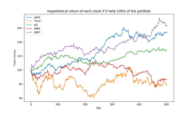
We can see that stocks like WMT and AAPL are performing well during this period, and we’d hope that Cover’s algorithm will upweight these stocks over the course of these days.
Now, let’s run Cover’s algorithm. Each day after observing the daily returns, we compute the weighted average over all portfolios, and rebalance the money accordingly. Initially, we start with a portfolio uniformly distributed across the stocks (20\% each). Note that we also discretize the space of portfolios into increments of 0.1 to be able to more easily compute the sum.
Here are the portfolio weights over time:
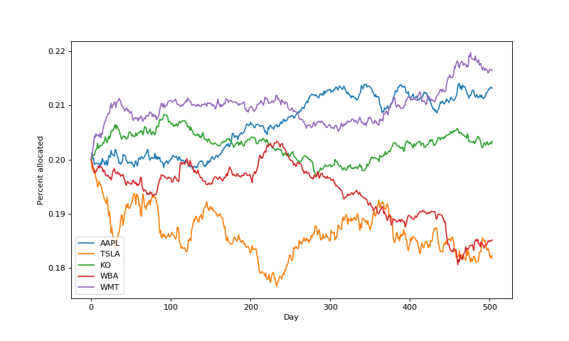
We can see that, indeed, the algorithm is allocating more money to the winning stocks, which is a nice sanity check. In fact, the portfolio weights largely mirror the performance of individual stocks above.
Now, let’s compare our results to the best porfolio in hindsight. It turns out that in this case $p^*$ allocates all of its money to the highest earning stock over the period, WMT.
Here are the earnings of each stock, along with those of Cover’s algorithm:
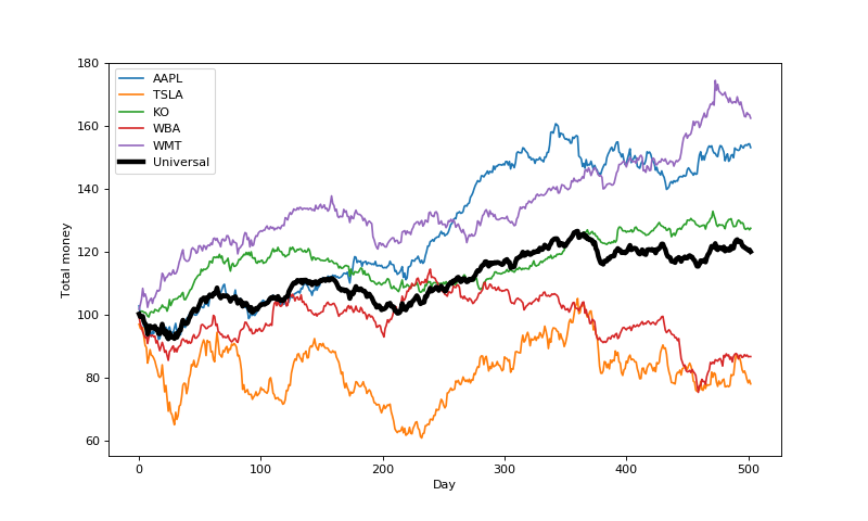
The universal portfolio algorithm is clearly making positive earnings, but it’s not clear that it’s approaching the best constant rebalanced portfolio (depicted as WMT in the plot above). A key question is how quickly we can expect the algorithm to converge to the best possible. Cover explores the specific rate of convergence in his paper, but we won’t get into it here.
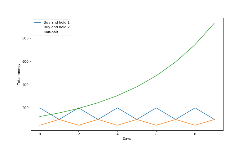
Also, note that the best constant rebalanced portfolio will not always be a “buy and hold” strategy (i.e., sticking with one stock) as it was in this case. If stocks fluctuate rapidly, it’s possible that a balance between the stocks is optimal. An example given in Elad Hazan’s book is the following two stock returns:
\[x_1 = \left( 2, \frac{1}{2}, 2, \frac{1}{2}, \dots \right)\] \[x_2 = \left( \frac{1}{2}, 2, \frac{1}{2}, 2, \frac{1}{2}, \dots \right)\]Sticking with only one of the stocks won’t make any money, but splitting and maintaining money half-and-half between them guarantees a daily return of 1.25. We can see this in the plot below:
Conclusions
Here, we introduced the idea of universal portfolios, and reviewed Thomas Cover’s simple algorithm for computing a daily portfolio. There has been a lot of work advancing these concepts since Cover’s initial paper, showing that more sophisticated online learning algorithms can provide even better guarantees in terms of rates of convergence and bounds on regret.
Code for the examples above can be found here.
References
- Cover, Thomas M. “Universal portfolios.” The Kelly Capital Growth Investment Criterion: Theory and Practice. 2011. 181-209.
- Hazan, Elad. “Introduction to online convex optimization.” Foundations and Trends® in Optimization 2.3-4 (2016): 157-325.
- This Quantopian post helped my implementation.