Thompson sampling

Thompson sampling is a simple Bayesian approach to selecting actions in a multi-armed bandit setting.

Multi-armed bandits

A multi-armed bandit is a sequential decision making problem. The name originally refers to a row of slot machines in a casino, each one with an arm that’s ready to take your money.

More precisely, in the multi-armed bandit setting, we have to choose an action at each timestep $t=1,2,\dots$. At each step, there are $K$ actions to choose from, $x_1, \dots, x_K$. After we choose an action $a_t \in {x_1, \dots, x_K}$, we receive a reward $r_t$. The goal is to maximize our reward over some (possibly infinite) time horizon:

Often, a discount factor, $\gamma \in [0, 1]$, is included so that more temporally distant rewards aren’t as beneficial as ones immediately in the future. In this case, the optimization problem becomes

Essentially, bandits are a special case of a Markov decision process (MDP), where the MDP only has one state. Recall that MDPs are made up of actions, rewards, and states (and a transition function describing probabilistically how an agent moves to different states). The agent in an MDP has the same goal as in a bandit setting: maximize reward. Bandits have been generalized to include state variables — often called “contextual bandits” — but we’ll focus on state-less bandits here.

Typically, the rewards earned from each action aren’t constant. Rather, we assume each action has some associated distribution over rewards, and when we choose an action, a reward is randomly sampled from this distribution. Below, we consider the simple case of a Bernoulli distribution, but the strategies described generalize to arbitrary distributions.

Bernoulli bandits

Here, we’ll focus on the special case where the rewards are always either $0$ or $1$. Specifically, we’ll assume that arm $k$’s reward is a Bernoulli random variable with parameter $\theta_k$. This means that if we choose action $k$ at step $t$, the reward is distributed as

with $r_t^k \in {0, 1}$. Recall that the Bernoulli PDF is

Clearly, if we knew the true values for ${\theta_k}$ a priori, then trivially the best strategy would be to always choose the arm with the highest expected value,

However, we virtually never know the true parameters in real-world scenarios, so we have to infer them from experience.

When $t=0$, we don’t know anything about the environment. Thus, for our first action, we can simply randomly select an arm, as they’re all exchangeable at this point.

As we try more arms and observe more rewards, we can update our expectation for how much reward we’ll get for each arm.

In this type of setting, there is a trade-off between exploitation and exploration. Exploitation refers to capitalizing on actions with known expected rewards. Exploration refers to trying new actions that we may know less about, but may have promise for even higher rewards.

Maximum likelihood solution

One strategy is to estimate $\widehat{\theta}_k$ at each timestep using its maximum likelihood estimate (MLE). Here, we initialize each parameter as $\theta_k = 0.5$ for all $k$. Then, at each time-step, we update each $\widehat{\theta}_k$ using its MLE (which is the sample average in this case):

where $n_k$ is the number of time-steps in which action $k$ was selected. Note that in practice, we only need to update the most recently-chosen arm’s parameter at each step.

Using the MLEs, our strategy is then to take the arm with the highest current estimate,

The advantage of this strategy is that it’s simple and computationally feasible for many distributional assumptions.

However, it’s sub-optimal and can lead to repeatedly choosing an arm whose expected reward is not the maximum among arms.

To see this, consider a scenario in which there are just two arms $a_1, a_2$ with true expected returns $\theta_1=0.8$ and $\theta_2 = 0.9$. Suppose we randomly choose $a_1$ as our first action and we observe $r_1=1$. Then the MLEs are $\widehat{\theta}_1^2 = 1, \widehat{\theta}_2^2 = 0.5$, so clearly we’ll choose $a_1$ again in the second round. If this continues, and it remains true that $\widehat{\theta}_1 > \widehat{\theta}_2$, then we’ll never choose $a_2$. However, this is sub-optimal because $a_2$ has a higher true expected reward.

To run a quick numerical experiment to show this, we can use the code below. It simulates a trajectory of a two-armed Bernoulli bandit using the MLE approach.

import numpy as np
import matplotlib.pyplot as plt
import seaborn as sns

# True parameters
theta_true = [0.8, 0.9]

# Runs one trajectory of the multi-armed bandit using MLE
def run_one_trajectory_mle(T=1000, save_trace=False):
    
    # Initialize estimates
    theta_hats = [0.5, 0.5]
    rewards = [[], []]
    if save_trace:
        trace = [theta_hats.copy()]
    
    # Run trajectory
    for t in range(T):
        
        # Choose an arm
        if theta_hats[0] == theta_hats[1]:
            action = np.random.choice([1, 2])
        else:
            action = np.argmax(theta_hats) + 1
            
        # Pull the arm and observe reward
        reward = np.random.binomial(n=1, p=theta_true[action-1])
        rewards[action-1].append(reward)
        
        # Update estimate
        theta_hats[action-1] = (theta_hats[action-1] * (t + 1) + reward) / (t + 2)
        
        if save_trace:
            trace.append(theta_hats.copy())
    
    if save_trace:
        return theta_hats, trace
    else:
        return theta_hats
        
# Run a bunch of trajectories
n_trajs = 1000
winners = []
for _ in range(n_trajs):
    theta_ests = run_one_trajectory_mle()
    winner = np.argmax(theta_ests) + 1
    winners.append(winner)

sns.countplot(winners)
plt.xlabel("Arm")
plt.ylabel("Win count")
plt.show()

Now, we can look at which arm had the highest $\widehat{\theta}$ at the end of the trajectory.

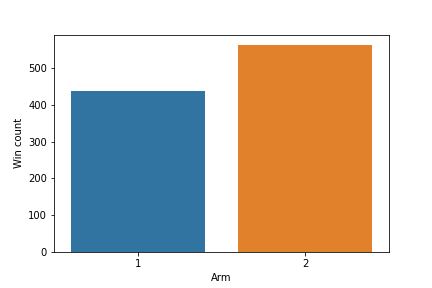
Even though arm $2$ is the true best choice, it only truly “wins” over arm $1$ a slight majority of the time.

We can also plot the estimates $\widehat{\theta}_1, \widehat{\theta}_2$ across two example trajectories. We can see that — even though the true expected reward is approached for one of the arms — the eventual winning arm depends heavily on the random behavior early on in the trajectory.

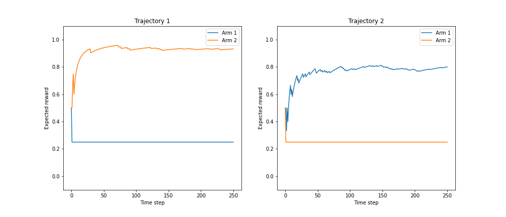
As we can see, the MLE approach is greedy — always selecting the arm with the highest current estimate of reward — and doesn’t allow for exploration. Next we’ll see that this issue is remedied by Thompson sampling.

Bayesian solution (Thompson sampling)

To alleviate these issues, another strategy would be to take a Bayesian approach to estimating the expected reward of each action. This allows us to mix in some uncertainty about the parameter estimates, which avoids getting stuck in a local optimum with greedy behavior.

Suppose we place a conjugate Beta prior on each Bernoulli parameter. For each arm, our model is now

\begin{align} r_t^k &\sim \text{Bern}(\theta_k) \\ \theta_k &\sim \text{Beta}(\alpha, \beta). \end{align}

Now, given some observed rewards for arm $k$, ${r_t^k}$, we can compute the posterior for $\theta_k$. Let $R^k_t = \sum\limits_{t : a_t = k} r_t$ be the total cumulative reward earned from arm $k$ up until time $t$, and let $n^k_t$ be the cumulative number of times arm $k$ was chosen. Then the posterior at time $t$ is

By updating the posterior at each step, we now have a distribution over each Bernoulli parameter. How do we then select an action using these distributions?

One idea would be to compute the mode of each distribution and choose the arm that has the highest mode. This would be equivalent to maximum a posteriori (MAP) estimation of the expected rewards. However, this would have the same issue as the MLE: we could get stuck in a local optimum.

A more flexible solution would be to use the posteriors as a means of exploration. Suppose we draw a random sample from each posterior at each time step, and take the arg-maximum as our selected action. This strategy is known as Thompson sampling, named after William R. Thompson.

Specifically, the algorithm works as follows. Let $\Pi_t^k$ be the posterior distribution for $\theta_k$ at time $t$. (This is just the prior when $t=0$.)

1. Sample $\widetilde{r}_t^k \sim \Pi_t^k$ for $k \in [K]$.
2. Take action $a_i$ where $i = \text{arg}\max_k r_t^k$, and observe reward $r_t^k$.
3. Update the posterior $\Pi_t^i$ with the new data point.

Below, we run another numerical experiment using Thompson sampling. This is again a two-armed Bernoulli bandit. Here is the code adapted for Thompson sampling:

def run_one_trajectory_thompson(T=1000, save_trace=False):
    
    # Initialize estimates
    alpha, beta = [1, 1], [1, 1]
    rewards = [[], []]
    if save_trace:
        trace_alpha = [alpha.copy()]
        trace_beta = [beta.copy()]
    
    # Run trajectory
    for t in range(T):
        
        # Choose an arm
        sample1 = np.random.beta(a=alpha[0], b=beta[0])
        sample2 = np.random.beta(a=alpha[1], b=beta[1])
        action = np.argmax([sample1, sample2]) + 1
            
        # Pull the arm and observe reward
        reward = np.random.binomial(n=1, p=theta_true[action-1])
        rewards[action-1].append(reward)
        
        # Update estimate
        alpha[action-1] = alpha[action-1] + reward
        beta[action-1] = beta[action-1] + 1 - reward
        
        if save_trace:
            trace_alpha.append(alpha.copy())
            trace_beta.append(beta.copy())
    
    if save_trace:
        return alpha, beta, trace_alpha, trace_beta
    else:
        return alpha, beta

We can again check which arm “wins” most of the time. Here, I plot the mean of the posterior distribution for each arm, which is given by the mean of a beta distribution:

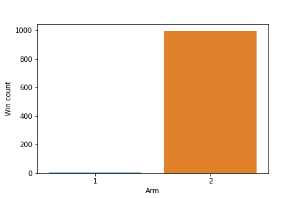
Clearly, using Thompson sampling, arm $2$ (the truly best arm) becomes the eventual winner the vast majority of the time.

We can also examine the evolution of the posterior mean across an example trajectory:

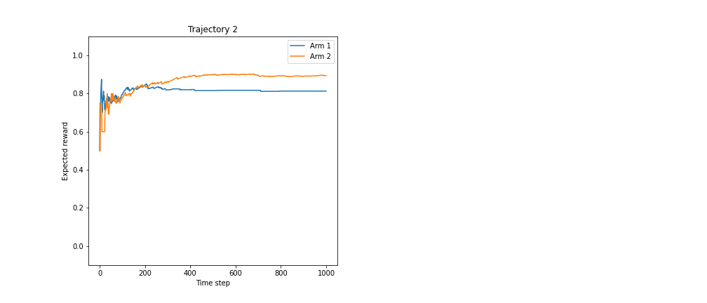
Here, both arms’ estimates approach their true parameter values.

Conclusion

Thompson sampling is attractive due to its simplicity and reliability. It is tractable as long as the posterior can be computed or approximated. It also provides a principled way to balance exploration and exploitation. There are deeper connections between Thompson sampling and other bandit strategies — such as upper confidence bound (UCB) methods — that I hope to explore in other posts.

References

• Russo, Daniel, et al. “A tutorial on thompson sampling.” arXiv preprint arXiv:1707.02038 (2017).