Andy Jones
Wiener and Ito processes
A brief review three types of stochastic processes: Wiener processes, generalized Wiener processes, and Ito processes.
Wiener processes
A random variable $z$ that follows a Wiener process (also known as Brownian motion) has two properties:
- For any interval of time $\Delta t$, the following holds: \(\Delta z = \epsilon \sqrt{\Delta t}\) where $\epsilon \sim \mathcal{N}(0, 1)$.
- Any two time intervals $\Delta t^{(1)}$ and $\Delta t^{(2)}$ obey the Markov property. That is, the correspoding changes in $z$ are independent.
Consider a random variable $y \sim \mathcal{N}(\mu, \sigma^2)$. Then recall that for any constant $c$, it holds that $cy \sim \mathcal{N}(\mu, c^2 \sigma^2)$. Applying this fact to point (1) above, we know that \(\Delta z \sim \mathcal{N}(0, \Delta t).\)
Consider $n$ discrete time intervals of length $\Delta t$. Recall that the variance of independent Gaussian random variables is additive. To see this, consider two RVs $X$ and $Y$ that have mean $0$ (without loss of generality. Then,
\begin{align} \mathbb{V}[X + Y] &= \mathbb{E}[(X + Y)^2] - \mathbb{E}[X + Y]^2 \\ &= \mathbb{E}[(X + Y)^2] - \underbrace{\mathbb{E}[X + Y]^2}_{0} \\ &= \mathbb{E}[X^2 + 2XY + Y^2] \\ &= \mathbb{E}[X^2] + \underbrace{\mathbb{E}[2XY]}_{0} + \mathbb{E}[Y^2] \\ &= \mathbb{E}[X^2] + \mathbb{E}[Y^2] \\ &= \mathbb{V}[X] + \mathbb{V}[Y] \end{align}
Thus, we know that \(\sum\limits_{i=1}^n \epsilon_i \sim \mathcal{N}(0, n \Delta t).\)
If we let $\Delta t \to 0$, then we can consider a continuous-time process, and we can write the corresponding process as
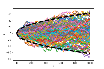
\[dz = \epsilon \sqrt{dt}.\]We can draw from a Wiener process with the following simple Python code. (Here, we necessarily make the process discrete so that we can sample on a computer.)
def draw_wiener_process(n=100):
    x = [np.random.normal()]
    for ii in range(1, n):
        x.append(x[ii - 1] + np.random.normal())
    return x
An example of 100 draws from this process is plotted below. The dashed black lines denote twice the standard deviation of the process at each time point, which contain about 95\% of the processes (based on the properties of the Gaussian).
Generalized Wiener process
The generalized Wiener process is a Wiener process that is allowed to have a mean and variance different than $0$ and $1$, respectively. It has the form \(dx = a dt + b dz.\) The term $a dt$ allows for a consistent linear change in the mean over time, while the term $b dz$ is a scaled Wiener process.
In other words, we can think about the generalized Wiener process as having the same form as the Wiener process \(\Delta x = \epsilon \sqrt{\Delta t}\) where now \(\epsilon \sim \mathcal{N}(a, b^2).\) This implies that for any time length $\Delta t$, the corresponding change in $x$, $\Delta x$ satisifies $\mathbb{E}[\Delta x] = a$ and $\mathbb{V}[\Delta x] = b^2 \Delta t$.
We can draw from a generalized Wiener process by simply adding a mean and standard deviation to the Wiener process above:
def draw_generalized_wiener_process(mu, sigma, n=100):
    x = [np.random.normal()]
    for ii in range(1, n):
        x.append(x[ii - 1] + np.random.normal(loc=mu, scale=sigma))
    return x
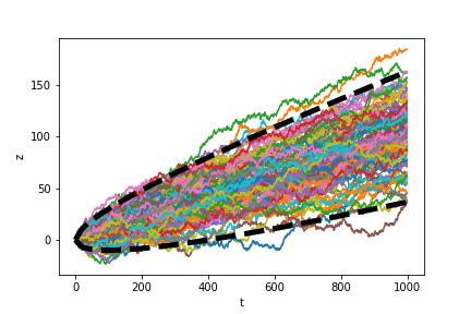
We plot 100 draws of a generalized Wiener process with $a = 0.1$ and $b = 1$ below.
Ito process
The Ito process generalizes the Wiener process further by allowing $a$ and $b$ to be functions of the variable $x$. It has the form \(dx = a(x, t) dt + b(x, t) dz\) where $z$ is a Wiener process.
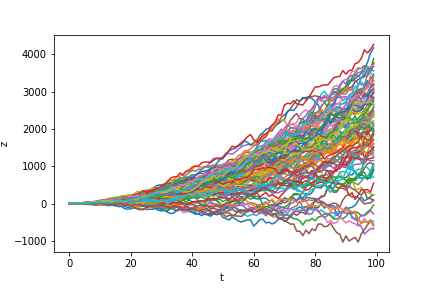
As a simple example, consider the case when \(a(x, t) = [\max(0, x)]^{1/2}\) and \(b(x, t) = \max(1, t).\)
We can simulate an Ito process in Python with the following code (here, $f$ and $g$ are assumed to be lambda functions in Python):
def draw_ito_process(f, g, n=100):
    x = [1]
    for ii in range(1, n):
        curr_x = x[ii - 1] + np.random.normal(loc=f(x[ii-1], ii), scale=g(x[ii-1], ii))
        x.append(curr_x)
    return x
In the draws below, we see that if the path’s trajectory remains positive, it has higher growth than if it veers into negative territory (due to the exponential mean function in $a$).
References
- Hull, John. Options, futures and other derivatives/John C. Hull. Upper Saddle River, NJ: Prentice Hall,, 2009.
- Prof. David Gamarnik’s notes on Ito Processes and Ito’s formula.