Regression splines

\(\DeclareMathOperator*{\argmin}{arg\,min}\) \(\DeclareMathOperator*{\argmax}{arg\,max}\)

Fitting smooth, nonlinear curves through data is a central aspect of analyzing complex datasets. However, nonlinear regression methods are often computationally demanding and can be much more prone to overfitting to simpler linear models.

Regression splines aim to solve some of these problems by fitting different curves for different regions of the input space. In this post, we’ll review some of the basics behind regression splines, as well as a special edge case of regression splines called smoothing splines.

Splines: A brief history

The word “spline” dates back to at least the 19th century, when it referred to a flexible piece of material used to draw curves for engineering and artistic purposes. The spline could be bent into a certain curved shape and held in place by placing pins at certain locations along the spline.

One of the most common uses of splines was for designing watercraft; a spline could be used to ensure a smooth curve for the bow in a sketch of a boat. For example, in his 1889 book Canoe and Boat Building: A Complete Manual for Amateurs, William Picard Stephens explains how to use a spline to draw a model sketch for a boat:

Taking a long spline, we will lay it on the drawing so as to pass through these three spots, confining it by lead weights or by small pins on either side of it at each point. If it does not take a “fair” curve without any abrupt bends, other pins or weights must be added at various points until it is true and fair throughout, when the line may be drawn in with a pencil.

The image below (courtesy of the Wikipedia entry for splines) shows an example of such a spline with two pins in the middle to create an S-like curve. The artist or engineer can then trace along the spline with a pen or pencil to create a smooth curve.

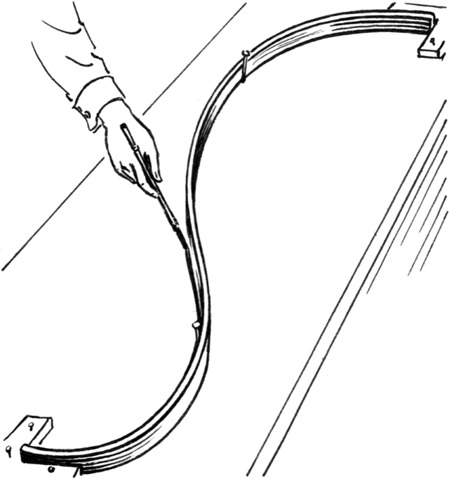
In the image above, we can see that the locations of the two pins determine the shape of the curve. As we’ll see next, there’s a direct analog for splines in statistics too.

Linear modeling

Before we introduce regression splines, let’s review some basics behind linear modeling.

Consider a regression problem where we observe $n$ input-output data pairs $\{(\mathbf{x}_i, y_i)\}_{i=1}^n$ and we would like to fit a function $f : \mathcal{X} \rightarrow \mathcal{Y}$ that describes the relationship between inputs and outputs. In this post, we’ll assume $\mathbf{x}_i \in \mathcal{X} = \mathbb{R}^p$ and $y \in \mathcal{Y} = \mathbb{R}$. (In most examples here, we will assume $p=1.$) For ease of notation, we’ll also write the data in matrix form as $\mathbf{X} = (\mathbf{x}_1, \cdots, \mathbf{x}_n)^\top \in \mathbb{R}^{n \times p}$ and $\mathbf{y} = (y_1, \cdots, y_n)^\top \in \mathbb{R}^n.$

A (ridge-regularized) linear model solves the following optimization problem:

where $\lambda \geq 0$ is a tuning parameter controlling the strength of regularization, and $|\cdot|_2$ denotes the $L_2$ norm of a vector. This problem has a well-known closed-form solution:

When $\lambda=0$, we recover the classic ordinary least squares (OLS) solution for the linear regression problem.

Piecewise regression

The linear modeling framework is often too inflexible to be able to capture complex trends in many datasets. Thus, there is often a need to turn to nonlinear models that can fit a smooth curve through the data.

A popular class of nonlinear regression functions are splines. There are several different subclasses of splines, but the basic unifying idea behind all of them is to fit a function locally within each region of the domain, and then connect these functions to yield a regression function that is nonlinear (and smooth) globally across the domain.

Many regression spline variations include a set of “knots” $\tau_1, \dots, \tau_K.$ Between any two adjacent knots, $\tau_k$ and $\tau_{k + 1},$ these approaches fit a local function using data from that interior region. Within each of these regions, we can then use a standard basis expansion to model nonlinear trends. A common choice for the basis expansion is a polynomial of degree $D.$ For a univariate sample $x,$ a $D$-degree polynomial expansion is given by

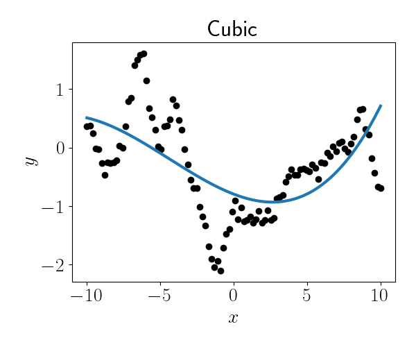
To motivate regression splines, consider the data below (black dots), along with the fit of a cubic polynomial globally to the data (blue line). It’s clear that a single cubic polynomial to the entire dataset is failing to capture the full regression trend.

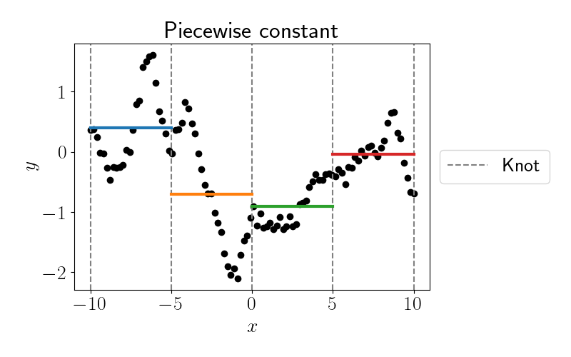
Regression splines attempt to remedy this by fitting functions within each local region of the domain. Suppose we use five knots at locations $\{-10, -5, 0, 5, 10\}.$ Then between each of these knots we can fit a polynomial of degree $D.$ Before we move to fully smooth splines, let’s start with a piecewise constant model (i.e., $D=0$), whose fit is shown below.

Let’s now move to a simple linear model in each region (i.e., $D=1$). The fits are shown below.

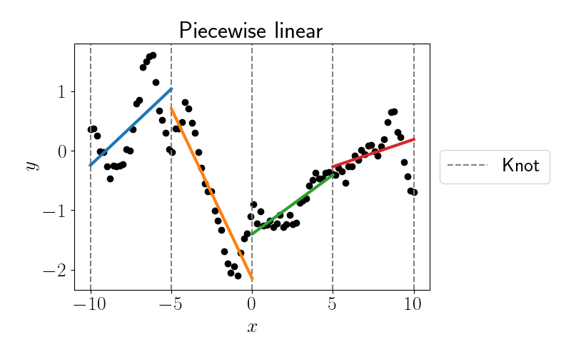
Again, clearly a piecewise linear model is failing to capture the nonlinearity within each inter-knot region. Let’s try bumping it up to a piecewise quadratic function (i.e., $D=2$).

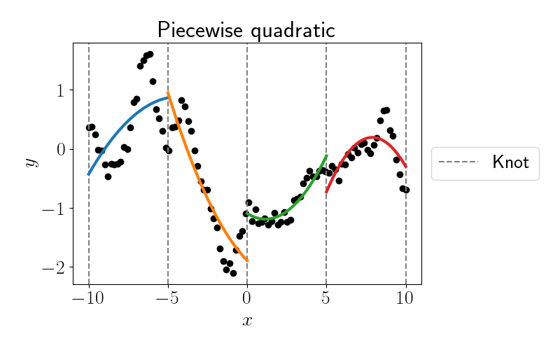
Getting better, but still not quite right. Let’s try one more with piecewise cubic fits (i.e., $D=3$).

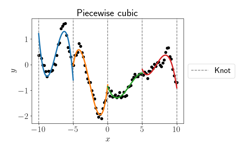
This one looks best of all, but clearly it’s still failing in some ways. We could continue to fit higher-degree polynomials, but we’ll stop this demonstration for now.

A major pathology to notice in all of the above examples is the discontinuity at the knots. In this naive approach to piecewise regression, we didn’t force the functions to be continuous or or have continuous derivatives at the knot locations. This could be a big issue for interpolation and prediction, and fortunately regression splines are designed to fix this issue, as we’ll see below.

Let’s now move to our discussion of two types of regression spline models: regression splines and smoothing splines.

Regression splines

The idea behind regression splines is to tranform the design matrix $\mathbf{X}$ with a particular set of basis functions, and then the same OLS fitting methods can be used with the transformed design matrix.

To begin a regression spline modeling approach, we first choose the locations of a set of “knots” $\tau_1, \dots, \tau_K.$ Between any two adjacent knots, $\tau_k$ and $\tau_{k + 1},$ we will fit a local function using data from that interior region. However, unlike before, we’ll now constrain the function at the knots to be continuous and possibly have some number of continuous derivatives.

Linear example

To see how continuity is enforced, let’s consider a simple example: fitting a piecewise linear function that is constrained to be continuous at the knot locations (unlike our piecewise linear fit above). Consider the dataset below, where we now just have one knot. Suppose we take an iterative approach to fitting a function, where we fit a linear model for each inter-knot region sequentially, constraining subsequent fits to be continuous with previous fits. Below, we perform one step of this by fitting a linear model only for the data to the left of the knot.

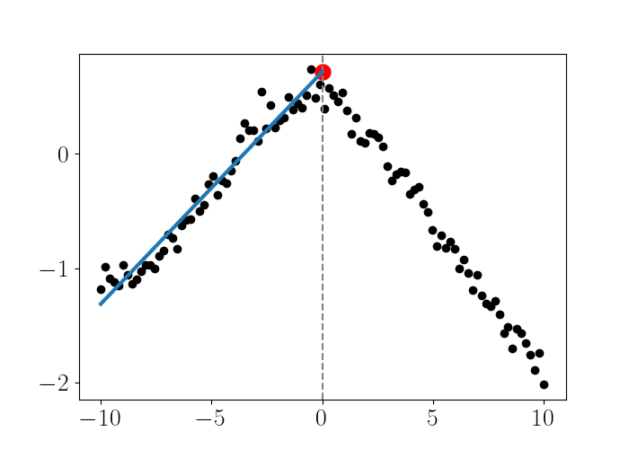
Now for the data to the right of the knot, we want to enforce that the linear fit for this data intersects the knot $\tau_1 = 0$ at the same location as the linear fit for the left side (shown by the red dot).

Notice that to enforce this constraint, we essentially have to force the “intercept” at $\tau_1$ to be the same for both linear fits, while allowing the slopes to be different. We can do this by adding a basis function that only takes into account the data to the right of the knot $\tau_1$. This function is given by

where $a_+ = \text{max}(0, a).$ We plot this fit below.

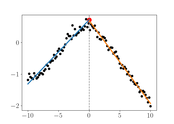
And here is the code to reproduce this fit:

import numpy as np
from scipy.stats import multivariate_normal as mvn
from sklearn.gaussian_process.kernels import RBF

np.random.seed(5)

lim = 10
n = 100
noise_variance = 1e-2
kernel = RBF(length_scale=6)
X = np.linspace(-lim, lim, n).reshape(-1, 1)
K = kernel(X) + np.eye(n) * noise_variance
Y = mvn.rvs(mean=np.zeros(n), cov=K)

knot_locs = [0]

def linear_spline_basis(X, knot_locations):

    X_expanded = np.hstack(
        [
            np.ones(X.shape),
            X,
            *[np.maximum(X - kl, 0) for kl in knot_locations],
        ]
    )
    return X_expanded

X_basis_expanded = linear_spline_basis(X, knot_locs)
beta = np.linalg.solve(X_basis_expanded.T @ X_basis_expanded, X_basis_expanded.T @ Y)

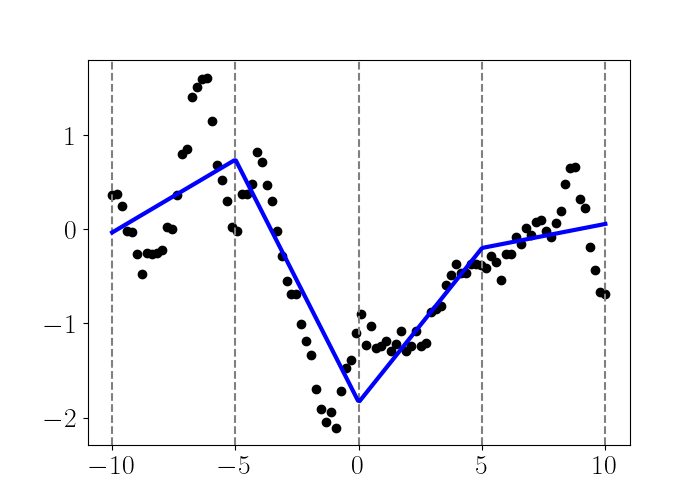
To accommodate more knots, we can add a new basis function of the form $\phi_{k}(x) = (x - \tau_k)_+^3$ for knots $k=1,\dots,K.$ Turning back to our dataset from the start of the post, we can fit a linear regression spline with those five knots:

Cubic splines

A more common choice for the basis expansion is a cubic polynomial. For a univariate sample $x,$ the basis functions for a cubic polynomial are given by

Now, to enforce the constraint that the function is continuous at the knot locations, we have to add other basis functions as well. In particular, to force the function to be continuous, as well as have continuous first and second derivatives, we add the following $K$ basis functions:

where, again, $a_+ = \text{max}(0, a).$

To try this, let’s fit a cubic regression spline with the same data as before. Here’s a snippet of Python code that runs this experiment:

import numpy as np
import matplotlib.pyplot as plt
from scipy.stats import multivariate_normal as mvn
from sklearn.gaussian_process.kernels import RBF


np.random.seed(10)

lim = 10
n = 100
noise_variance = 1e-2
kernel = RBF()
X = np.linspace(-lim, lim, n).reshape(-1, 1)
K = kernel(X) + np.eye(n) * noise_variance
Y = mvn.rvs(mean=np.zeros(n), cov=K)

knot_locs = [-lim + 1, -lim / 2, 0, lim / 2, lim - 1]

def cubic_spline_basis(X, knot_locations):

    X_expanded = np.hstack(
        [
            np.ones(X.shape),
            X,
            X ** 2,
            X ** 3,
            *[np.maximum(X - kl, 0) ** 3 for kl in knot_locations],
        ]
    )
    return X_expanded

# Basis expansion
X_basis_expanded = cubic_spline_basis(X, knot_locs)

# Fit OLS with expanded basis
beta = np.linalg.solve(X_basis_expanded.T @ X_basis_expanded, X_basis_expanded.T @ Y)

We can then plot the function across the domain, as shown below. Note that predictions are easily made with splines by simply using our fitted beta by calling X_test @ beta in Python.

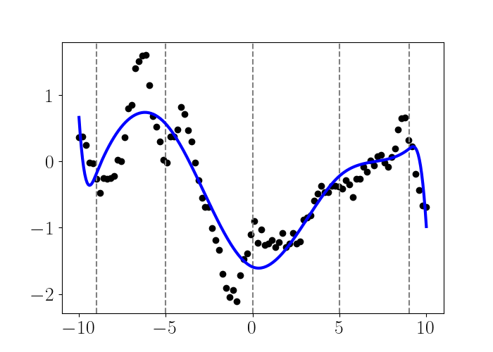
We can see that this approach fits a smooth function through the data, and there are no visible jumps at the knot locations.

Other spline bases have also been discovered, such as the B-spline (basis spline), that are more computationally efficient when the number of knots is large. The B-spline basis has nice theoretical properties, such as the fact that it’s a basis for all cubic polynomials with a particular set of knots.

Smoothing splines

Smoothing splines can be seen as a certain limiting case of regression splines when we select the maximum number of knots, i.e., the number of knots is equal to the number of data points. Notice that when we allow the maximum number of knots, $K=n,$ and fit the model with OLS as we did above, we will get a function that perfectly interpolates the data. However, because this function is only very loosely constrained, the function can be very “wiggly” and overfit to the data. To see this, here’s a cubic spline fit to the same dataset as above with a knot placed at each data point:

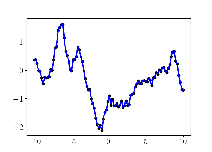
This approach effectively assumes that the data is noiseless. In fact, spline functions were first introduced as a way of exactly interpolating a set of points; in other words, they were introduced under the assumption of zero noise. This construction, which was largely from the mathematics community, sought a function $f$ with the restriction that $y = f(x_i).$

However, the statistics community is much more interested in smoothing than interpolation. Specifically, we can assume that there is some measurement noise $\epsilon$ and our observations are no the true function value, $y = f(x) + \epsilon.$ If we search for a function that exactly interpolates these noisy observations, it will be horridly overfit and curvy (especially if it’s a high-degree polynomial). Instead, we need to account for the noise directly.

To fix this overfitting issue, a common approach is to regularize the “curviness” of the function directly. This is commonly done by penalizing the second derivative of the function. This approach yields the following minimization problem for smoothing splines:

\begin{equation} \min_{f \in \mathcal{F}} \underbrace{\sum\limits_{i=1}^n (y_i - f(x_i))^2}_{\text{Error}} + \underbrace{\lambda \int (f’‘(x))^2 dx}_{\text{Regularization}}, \label{eq:smoothing_spline} \tag{1} \end{equation}

where $\mathcal{F}$ is the set of all functions with two continuous derivatives. This minimization problem seeks a function $f$ that minimizes the distance to the data (first term) and is also not too wiggly (second term). The hyperparameter $\lambda$ controls the strength of the regularization. When $\lambda=0,$ we obtain an unregularized problem, and when $\lambda=\infty,$ any nonzero second derivative is not tolerated, so $f$ must be linear.

While the integral in Equation \ref{eq:smoothing_spline} may not always be tractable, we can often approximate it with finite differences (e.g., see here).

References

• Stephens, William Picard. Canoe and Boat Building: A Complete Manual for Amateurs. New York: Forest and Stream (1889).
• Schoenberg, I. J. “Cardinal interpolation and spline functions.” Journal of Approximation theory 2.2 (1969): 167-206.
• Hastie, Trevor, et al. The elements of statistical learning: data mining, inference, and prediction. Vol. 2. New York: springer, 2009.