Slice sampling

Slice sampling is a method for obtaining random samples from an arbitrary distribution. Here, we walk through the basic steps of slice sampling and present two visual examples.

Slice sampling

Consider an arbitrary probability density function $f(x)$. Given the current position of the sampler $x_t$ (or possibly the initial position when $t=0$), slice sampling consists of two main steps:

Draw a point $\hat{y}$ uniformly at random from the interval $[0, f(x_t)]$.
Draw the next sample $x_{t+1}$ uniformly at random from the set $\{x \; : \; f(x) > \hat{y}\}$.

Repeating this process many times will generate a set of samples $x_1, x_2, \dots$ such that their distribution will approach the true density of $f(x)$.

Examples

Standard normal

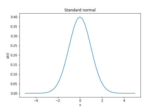
To start, consider a very simple target distribution: the standard normal distribution $\mathcal{N}(0, 1)$.

standard_normal_slice

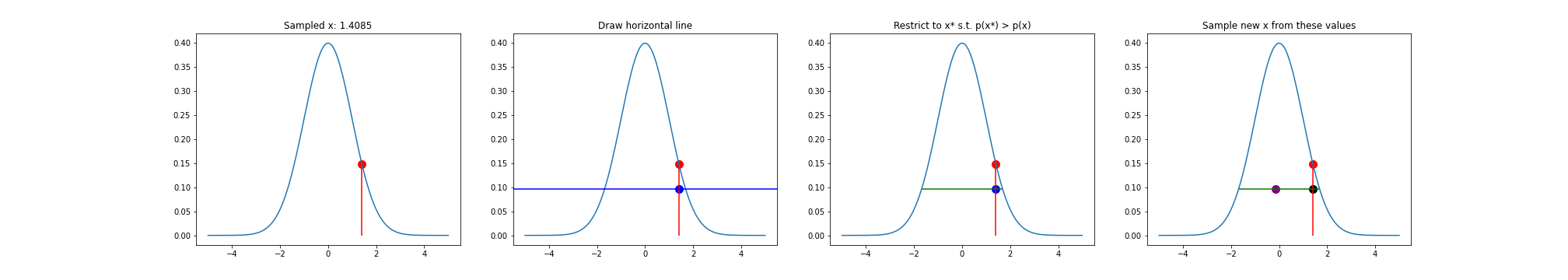
The four images below demonstrate the steps of slice sampling visually.

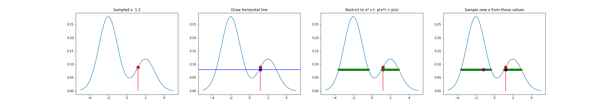
In the leftmost plot, we start with an initial value $x$, with corresponding density value $f(x)$. In the second plot, we randomly sample a new point along the vertical red line (this red line is the interval $[0, f(x)]$). The new point is the blue dot. In the third plot, we restrict the $x^\star$-values such that $f(x^\star) > f(x)$ — these values are presented as a horizontal green line. Finally, in the last plot on the right we randomly sample a point from this green interval (shown as a purple dot), treating this as our next sample. We can then repeat the process with this point.

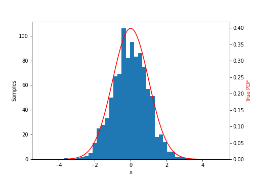
After running this process many times, we can see that the histogram of the samples $x_1, x_2, \dots, x_n$ approaches a standard normal.

Mixture of normals

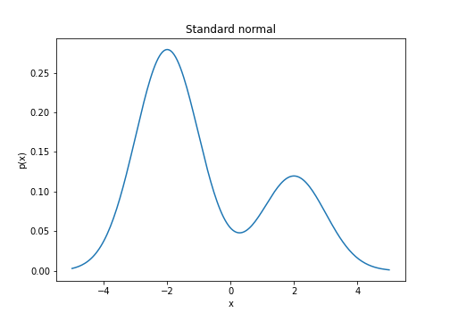
Now let’s examine a slightly more complex example: a mixture of two normal distributions. Specifically, let the target distribution be

\[f(x) = \pi_1 f_1(x) + \pi_2 f_2(x)\]

where

\begin{align} f_1(x) &= \mathcal{N}(-2, 1) \\ f_2(x) &= \mathcal{N}(2, 1) \\ \pi_1 &= 0.7 \\ \pi_2 &= 0.3. \\ \end{align}

The density looks like this:

standard_normal_slice

Plotting the same sequence of figures as above, we can see that the slice sampler hops between the two densities. For example, in the rightmost plot, the new sample (purple dot) is in the opposite mode of the previous sample.

Conlusion

Slice sampling is a nice, intuitively-appealing way to generate random samples from a distribution. Note that the version of slice sampling presented here is a simplification of that proposed by Neal. For example, to find the values of $x$ such that $f(x) > \hat{y}$ (step 2 above), Neal proposes a “stepping out” approach, while I used a naive sampling approach.

One major drawback of slice sampling is that the samples are serially dependent, which suggests that the Markov chain may take longer to converge than methods that produce independent samples.

Several extensions of slice sampling have been proposed, including elliptical slice sampling, which is specifically useful for statistical models with multivariate Gaussian priors.

Code

Code for generating these figures is below.

import numpy as np
import matplotlib.pyplot as plt
from scipy.stats import norm

#### Run one iteration of slice sampling for a standard normal ####

plt.figure(figsize=(28, 5))
# Pick an x randomly
x = norm.rvs()

# Evaluate density at this x
p_x = norm.pdf(x)

plt.subplot(141)
xs_plot = np.linspace(left_endpoint, right_endpoint, 200)
ys_plot = norm.pdf(xs_plot)
plt.plot(xs_plot, ys_plot)
plt.vlines(x, ymin=0, ymax=p_x, colors="red")
plt.scatter(x, p_x, c="red", s=100)
plt.title("Sampled x: {}".format(round(x, 4)))

# Pick a y uniformly at random from [0, f(x)]
y = np.random.uniform(low=0, high=p_x)

plt.subplot(142)
xs_plot = np.linspace(left_endpoint, right_endpoint, 200)
ys_plot = norm.pdf(xs_plot)
plt.plot(xs_plot, ys_plot)
plt.vlines(x, ymin=0, ymax=p_x, colors="red")
plt.scatter(x, p_x, c="red", s=100)
plt.scatter(x, y, c="blue", s=100)
plt.axhline(y, c="blue")
plt.title("Draw horizontal line")

# Find all x values such that f(x) > y
xs = np.linspace(left_endpoint, right_endpoint, 1000)
newxs = xs[norm.pdf(xs) > y]

plt.subplot(143)
plt.plot(xs_plot, ys_plot)
plt.vlines(x, ymin=0, ymax=p_x, colors="red")
plt.scatter(x, p_x, c="red", s=100)
plt.scatter(x, y, c="blue", s=100)
# plt.axhline(y, c="blue")
plt.hlines(y, xmin=np.min(newxs), xmax=np.max(newxs), colors="green")
plt.title("Restrict to x* s.t. p(x*) > p(x)")

# Choose new x uniformly at random from this set
newx = np.random.choice(newxs)
p_newx = norm.pdf(newx)

plt.subplot(144)
plt.plot(xs_plot, ys_plot)
plt.vlines(x, ymin=0, ymax=p_x, colors="red")
plt.scatter(x, p_x, c="red", s=100)
plt.hlines(y, xmin=np.min(newxs), xmax=np.max(newxs), colors="green")
plt.scatter(newx, y, c="purple", s=100)
plt.scatter(x, y, c="black", s=100)
plt.title("Sample new x from these values")

# Add this x to the set of sampled values
x = newx
samples.append(x)

plt.show()


#### Run multiple iterations of slice sampling for standard normal #####

NUM_SAMPLES = 1000
samples = []

for _ in range(NUM_SAMPLES):

    # Pick an x randomly
    x = norm.rvs()

    # Evaluate density at this x
    p_x = norm.pdf(x)

    # Pick a y uniformly at random from [0, f(x)]
    y = np.random.uniform(low=0, high=p_x)

    # Find all x values such that f(x) > y
    xs = np.linspace(left_endpoint, right_endpoint, 1000)
    newxs = xs[norm.pdf(xs) > y]

    # Choose new x uniformly at random from this set
    x = np.random.choice(newxs)

    # Add this x to the set of sampled values
    samples.append(x)

fig, ax1 = plt.subplots(figsize=(7, 5))

ax2 = ax1.twinx()
ax1.hist(samples, 30)
ax2.plot(xs_plot, ys_plot, c="red")

ax1.set_xlabel('x')
ax1.set_ylabel('Samples')
ax2.set_ylabel('True PDF', color='r')
ax2.set_ylim(bottom=0)

plt.show()


#### Plot mixture of normals ####

def mixture_pdf(x, pi1=0.7, pi2=0.3):
    return pi1 * norm.pdf(x, loc=-2) + pi2 * norm.pdf(x, loc=2)

left_endpoint, right_endpoint = -5, 5


plt.figure(figsize=(7, 5))

xs = np.linspace(left_endpoint, right_endpoint, 200)
ys = mixture_pdf(xs)
plt.plot(xs, ys)

plt.xlabel("x")
plt.ylabel("p(x)")
plt.title("Standard normal")
plt.show()


####  Run one iteration of slice sampling for mixture of normals #####

plt.figure(figsize=(28, 5))
# Pick an x randomly
x = 1.2 #norm.rvs(loc=2, scale=0.2)



# Evaluate density at this x
p_x = mixture_pdf(x)

plt.subplot(141)
xs_plot = np.linspace(left_endpoint, right_endpoint, 200)
ys_plot = mixture_pdf(xs_plot)
plt.plot(xs_plot, ys_plot)
plt.vlines(x, ymin=0, ymax=p_x, colors="red")
plt.scatter(x, p_x, c="red", s=100)
plt.title("Sampled x: {}".format(round(x, 4)))

# Pick a y uniformly at random from [0, f(x)]
y = np.random.uniform(low=0, high=p_x)

plt.subplot(142)
xs_plot = np.linspace(left_endpoint, right_endpoint, 200)
ys_plot = mixture_pdf(xs_plot)
plt.plot(xs_plot, ys_plot)
plt.vlines(x, ymin=0, ymax=p_x, colors="red")
plt.scatter(x, p_x, c="red", s=100)
plt.scatter(x, y, c="blue", s=100)
plt.axhline(y, c="blue")
plt.title("Draw horizontal line")

# Find all x values such that f(x) > y
xs = np.linspace(left_endpoint, right_endpoint, 1000)
newxs = xs[mixture_pdf(xs) > y]

plt.subplot(143)
plt.plot(xs_plot, ys_plot)
plt.vlines(x, ymin=0, ymax=p_x, colors="red")
plt.scatter(x, p_x, c="red", s=100)
plt.scatter(x, y, c="blue", s=100)
plt.scatter(newxs, np.repeat(y, newxs.shape[0]), c="green")
plt.title("Restrict to x* s.t. p(x*) > p(x)")

# Choose new x uniformly at random from this set
newx = np.random.choice(newxs)
p_newx = norm.pdf(newx)

plt.subplot(144)
plt.plot(xs_plot, ys_plot)
plt.vlines(x, ymin=0, ymax=p_x, colors="red")
plt.scatter(x, p_x, c="red", s=100)
plt.scatter(newxs, np.repeat(y, newxs.shape[0]), c="green")
plt.scatter(newx, y, c="purple", s=100)
plt.scatter(x, y, c="black", s=100)
plt.title("Sample new x from these values")

# Add this x to the set of sampled values
x = newx
samples.append(x)

# Repeat

plt.show()    

References

Neal, Radford M. “Slice sampling.” Annals of statistics (2003): 705-741.
Wikipedia entry on slice sampling.