Shrinkage in ridge regression

A brief review of shrinkage in ridge regression and a comparison to OLS.

OLS review

Consider the regression problem

\[Y = X\beta + \epsilon\]

where $Y$ is an $n$-vector of responses, $X$ is an $n \times p$ matrix of covariates, $\beta$ is a $p$-vector of unknown coefficients, and $\epsilon$ is i.i.d. noise. We can estimate $\beta$ by minimizing the sum of squares:

\[\ell = \frac12 \|Y - X\beta\|^2_2.\]

Taking the derivative w.r.t. $\beta$, we have

\[\frac{\partial \ell}{\partial \beta} = -X^\top (Y - X\beta).\]

Setting to zero, we have $X^\top Y = X^\top X\beta$, which implies

\[\widehat{\beta} = (X^\top X)^{-1} X^\top Y.\]

MLE interpretation of OLS

Note that an equivalent solution can be found by maximizing the likelihood of the model

\[Y \sim \mathcal{N}(X\beta, \sigma^2 I_p).\]

Consider maximizing the log likelihood:

\[\text{arg}\max_\beta \log p(Y | X, \beta) = \text{arg}\max_\beta -\frac{p}{2} \log 2\pi -\frac{p}{2} \log \sigma^2 - \frac{1}{2\sigma^2} (Y - X\beta)^\top (Y - X\beta).\]

Ignoring constant terms, we have

\[\frac12 p \log \sigma^2 = \frac{1}{2\sigma^2} (Y^\top Y - Y^\top X\beta - \beta^\top X^\top Y + \beta^\top X^\top X\beta)\]

Taking a derivative w.r.t. $\beta$, we have

\begin{align} &\frac{\partial \ell}{\partial \beta} = 0 = \frac{1}{2\sigma^2} (- X^\top Y - X^\top Y + 2 X^\top X \beta) \\ \implies& X^\top X \beta = X^\top Y \\ \implies& \widehat{\beta}_{\text{MLE}} = (X^\top X)^{-1} X^\top Y \end{align}

Ridge regression

Consider instead maximizing the sum of squares with an additional $\ell_2$ penalty on $\beta$:

\[\min_\beta \frac12 \|Y - X\beta\|^2_2 + \frac{\lambda}{2} \|\beta\|_2^2.\]

Taking a derivative w.r.t. $\beta$,

\[-X^\top (Y - X\beta) + \lambda \beta = 0.\]

This implies that $X^\top X\beta + \lambda \beta = X^\top Y$, and thus $(X^\top X + \lambda I_p) \beta = X^\top Y$. The solution can easily be seen as

\[\widehat{\beta}_{\text{ridge}} = (X^\top X + \lambda I_p)^{-1} X^\top Y.\]

In other words, we add a small constant value $\lambda$ to the diagonal of the sample covariance $X^\top X$ before inverting it.

To see this another way, consider the SVD of $X$,

\[X = UDV^\top.\]

Plugging this into the ridge regression solution, we have

\begin{align} \widehat{\beta} &= (VDU^\top UDV^\top + \lambda I_p)^{-1} VDU^\top Y \\ &= (VD^2V^\top + \lambda I_p)^{-1} VDU^\top Y \\ &= (D^2 + \lambda I_p)^{-1} VDU^\top Y. \end{align}

The fitted values $X \widehat{\beta}$ are then

\begin{align} X \widehat{\beta} &= X (D^2 + \lambda I_p)^{-1} VDU^\top Y \\ &= UDV^\top (D^2 + \lambda I_p)^{-1} VDU^\top Y \\ &= UD (D^2 + \lambda I_p)^{-1} DU^\top Y \\ &= \sum\limits_{j=1}^p u_j \frac{d_j^2}{d_j^2 + \lambda} u_j^\top Y \end{align}

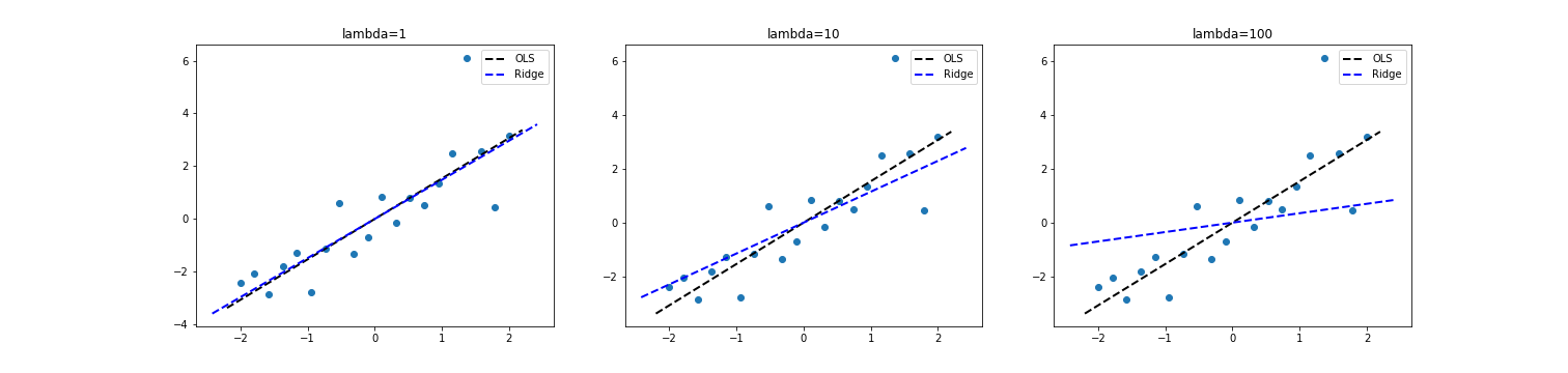
The “shrinkage factor” for feature $j$ is $\frac{d_j^2}{d_j^2 + \lambda}$. For mean-centered data, this essentially corresponds to a rotation of the coefficient vector toward zero. In effect, this means that the fitted values $\widehat{Y}$ are shrunk toward zero. Notice that if $\lambda=0$, it reduces to vanilla least squares with $X \widehat{\beta} = UU^\top Y$. This is the projection of Y onto the orthogonal subspace defined by $X$.

We can visualize this. Below is a scatter plot with $p=1$ and $n=20$ points where the true value $\beta=1.5$. As we plot the OLS and ridge estimates, we can see that the ridge coefficient rotates toward zero as $\lambda$ increases.

Furthermore, we can see that the shrinkage factor $\frac{d^2}{d^2 + \lambda}$ will decrease (causing more shrinkage) at the rate $\frac{c}{c + \lambda}$, where $c$ is a constant determined by the $j$th singular value of $X^\top X$:

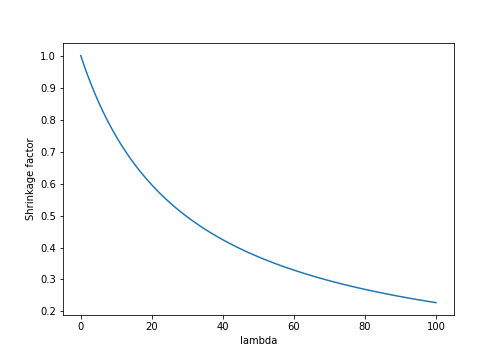
In higher dimensions, each covariate will have a different rate of shrinkage (determined by its corresponding singular value).

MLE interpretation of ridge regression

Notice that we can arrive at an equivalent solution to ridge regression assuming the following model, where we place a prior on $\beta$

\[Y \sim \mathcal{N}(X \beta, \sigma^2 I), ~~~ \beta \sim \mathcal{N}(0, \frac{1}{\lambda} I).\]

The posterior is

\[p(\beta | X, Y) = \frac1Z p(Y | X, \beta) p(\beta)\]

where $Z$ is the normalizing constant. We can find a MAP solution by maximizing the quantity without the constant, which is proportional to the posterior.

\begin{align} &\max_\beta \log p(Y | X, \beta) + \log p(\beta) \\ &= \max_\beta -\frac{p}{2} \log 2\pi -\frac12 p \log \sigma^2 - \frac{1}{2\sigma^2} (Y - X\beta)^\top (Y - X\beta) - \frac{p}{2} \log 2\pi -\frac{p}{2} \log \sigma^2 - \frac{\lambda}{2} |\beta|_2^2. \end{align}

Ignoring constant terms and taking a derivative w.r.t. $\beta$, we have

\begin{align} &-\frac{1}{2\sigma^2} \left( -X^\top Y - X^\top Y + 2 X^\top X \beta\right) -\frac{\lambda}{2} 2\beta = 0 \\ \implies& X^\top X \beta + \sigma^2 \lambda \beta = X^\top Y \\ \implies& \widehat{\beta} = \left( X^\top X + \sigma^2 \lambda I\right)^{-1} X^\top Y \end{align}

The ridge solution to collinearity

Suppose our data lives in $\mathbb{R}^2$, that is, $X \in \mathbb{R}^{n \times 2}$. Further, suppose the two columns of $X$ are identical. If we then perform linear regression with response $Y$, the problem is under-constrained: there are an infinite number of equally good solutions. To see this, consider an SVD of $X = UDV^\top$, and notice that

\[(X^\top X)^{-1} X^\top Y = UU^\top Y = \sum\limits_{j=1}^p u_j u_j^\top Y = u_1 u_1^\top Y + u_2 u_2^\top Y.\]

Since the columns of $X$ are equal, we know that $u_1 = u_2$. In this case, we can arbitrarily scale each term to get an infinite number of equivalent solutions:

\[\widehat{\beta} = \gamma u_1 u_1^\top Y + \frac{1}{\gamma} u_2 u_2^\top Y, ~~ \forall \gamma\in \mathbb{R}.\]

Ridge regression alleviates this issue by adding a small quantity to the diagonal of $X^\top X$ to make the solution unique:

\[u_1 \frac{d_1^2}{d_1^2 + \lambda} u_1^\top Y + u_2 \frac{d_2^2}{d_2^2 + \lambda} u_2^\top Y.\]