Andy Jones
The smoothly clipped absolute deviation (SCAD) penalty
Variable selection is an important part of high-dimensional statistical modeling. Many popular approaches for variable selection, such as LASSO, suffer from bias. The smoothly clipped absolute deviation (SCAD) estimator attempts to alleviate this bias issue, while also retaining a continuous penalty that encourages sparsity.
Penalized least squares
A large class of variable selection models can be described under the family of models called “penalized least squares”. The general form of these objective functions is
\[Q(\beta) = \frac1n ||\mathbf{Y} - \mathbf{X}\boldsymbol{\beta}||_2^2 + \sum\limits_{j = 1}^p p_\lambda(|\beta_j|)\]where $\mathbf{X} \in \mathbb{R}^{n\times p}$ is the design matrix, $\mathbf{Y} \in \mathbb{R}^n$ is the vector of response variables, $\boldsymbol{\beta} \in \mathbb{R}^p$ is the vector of coefficients, and $p_\lambda(\cdot)$ is a penalty function indexed by regularization parameter $\lambda$.
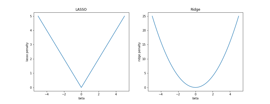
As special cases, notice that LASSO corresponds to a penalty function of $p_\lambda(\beta) = \lambda ||\beta||_1$, and ridge regression corresponds to $p_\lambda(\beta) = \lambda ||\beta||_2^2$. Recall the graphical shape of these univariate penalties below.
SCAD
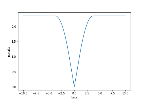
The smoothly clipped absolute deviation (SCAD) penalty, introduced by Fan and Li (2001), was designed to encourage sparse solutions to the least squares problem, while also allowing for large values of $\beta$. The SCAD penalty is part of a larger family known as “folded concave penalties”, which are concave on $\mathbb{R}_+$ and $\mathbb{R}_-$. Graphically, the SCAD penalty looks like this:
Somewhat oddly, the SCAD penalty is often defined primarily by its first derivative $p’(\beta)$, rather than $p(\beta)$. Its derivative is
\[p'_\lambda(\beta) = \lambda \left\{ I(\beta \leq \lambda) + \frac{(a\lambda - \beta)_+}{(a - 1) \lambda} I(\beta > \lambda) \right\}\]where $a$ is a tunable parameter that controls how quickly the penalty drops off for large values of $\beta$, and the function $f(z) = z_+$ is equal to $z$ if $z \geq 0$, and $0$ otherwise. We can gain some insight by breaking down the penalty function’s derivative for different values of $\lambda$:
\begin{cases} \lambda & \text{if } |\beta| \leq \lambda \\ \frac{(a\lambda - \beta)}{(a - 1) } & \text{if } \lambda < |\beta| \leq a \lambda \\ 0 & \text{if } |\beta| > a \lambda \\ \end{cases}
Notice that for large values of $\beta$ (where $|\beta| > a \lambda$), the penalty is constant with respect to $\beta$. In other words, after $\beta$ becomes large enough, higher values of $\beta$ aren’t penalized more. This stands in contrast to the LASSO penalty, which has a monotonically increasing penalty with respect to $|\beta|$:
\[p_\text{LASSO}(\beta) = |\beta|\] \[p'_\text{LASSO}(\beta) = \text{sign}(\beta)\]Unfortunately, this means that for large coefficient values, their LASSO estimates will be biased downwards.
On the other end, for small values of $\beta$ (where $|\beta| \leq \lambda$), the SCAD penalty is linear in $\beta$. And for medium values of $\beta$ (where $\lambda < |\beta| \leq a \lambda$), the penalty is quadratic.
Defined piecewise, $p_\lambda(\beta)$ is
\begin{cases} \lambda |\beta| & \text{if } |\beta| \leq \lambda \\ \frac{a \lambda |\beta| - \beta^2 - \lambda^2}{a - 1} & \text{if } \lambda < |\beta| \leq a \lambda \\ \frac{\lambda^2(a + 1)}{2} & \text{if } |\beta| > a \lambda \\ \end{cases}
In Python, the SCAD penalty and its derivative can be defined as follows:
def scad_penalty(beta_hat, lambda_val, a_val):
    is_linear = (np.abs(beta_hat) <= lambda_val)
    is_quadratic = np.logical_and(lambda_val < np.abs(beta_hat), np.abs(beta_hat) <= a_val * lambda_val)
    is_constant = (a_val * lambda_val) < np.abs(beta_hat)

    linear_part = lambda_val * np.abs(beta_hat) * is_linear
    quadratic_part = (2 * a_val * lambda_val * np.abs(beta_hat) - beta_hat**2 - lambda_val**2) / (2 * (a_val - 1)) * is_quadratic
    constant_part = (lambda_val**2 * (a + 1)) / 2 * is_constant
    return linear_part + quadratic_part + constant_part

def scad_derivative(beta_hat, lambda_val, a_val):
    return lambda_val * ((beta_hat <= lambda_val) + (a_val * lambda_val - beta_hat)*((a_val * lambda_val - beta_hat) > 0) / ((a_val - 1) * lambda_val) * (beta_hat > lambda_val))
Fitting models with SCAD
One general approach for fitting penalized least squares models (including SCAD-penalized models) is to use local quadratic approximations. This approach amounts to fitting a quadratic function $q(\beta)$ around an initial point $\beta_0$ such that the approximation:
- Is symmetric about 0,
- Satisfies $q(\beta_0) = p_\lambda(|\beta_0|)$,
- Satisfies $q’(\beta_0) = p’_\lambda(|\beta_0|)$.
Thus, the approximation function must have the form
\[q(\beta) = a + b \beta^2\]for coefficients $a$ and $b$ that don’t depend on $\beta$. The constraints above give us a system of two equations that we can solve:
- $a + b \beta_0^2 = p_\lambda(|\beta_0|)$
- $2b \beta_0 = p’_\lambda(|\beta_0|)$
For completeness, let’s walk through the solution. Rearranging the second equation, we have
\[b = \frac{p'_\lambda(|\beta_0|)}{2 |\beta_0|}.\]Plugging this into the first equation, we have
\begin{align} &a + \frac{p’_\lambda(|\beta_0|)}{2 |\beta_0|} \beta_0^2 = p_\lambda(|\beta_0|) \\ \implies& a = p_\lambda(|\beta_0|) - \frac{p’_\lambda(|\beta_0|)}{2 |\beta_0|} \beta_0^2 \end{align}
Thus, the full quadratic equation is
\begin{align} q(\beta) &= p_\lambda(|\beta_0|) - \frac{p’_\lambda(|\beta_0|)}{2 |\beta_0|} \beta_0^2 + \frac{p’_\lambda(|\beta_0|)}{2 |\beta_0|} \beta^2 \\ &= p_\lambda(|\beta_0|) + \frac{p’_\lambda(|\beta_0|)}{2 |\beta_0|} (\beta^2 - \beta_0^2) \\ \end{align}
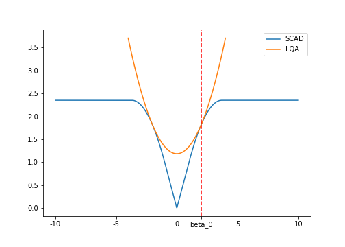
Now, for any initial guess $\beta_0$ for the coefficient value, we can constsruct a quadratic estimate of the penalty using $q$ above. Then, it’s much easier to find the minimum of this quadratic compared to the initial SCAD penalty.
Graphically, the quadratic approximation looks like this:
Putting the quadratic approximation to the SCAD penalty into the the full least-squares objective function, the optimization problem becomes:
\[\text{arg}\min_\beta Q(\beta) = \min_\beta \left[\frac1n ||Y - X \beta||_2^2 + p_\lambda(|\beta_0|) + \frac{p'_\lambda(|\beta_0|)}{2 |\beta_0|} (\beta^2 - \beta_0^2) \right].\]Ignoring the terms that don’t depend on $\beta$, this minimization problem is equivalent to
\[\text{arg}\min_\beta \left[\frac1n ||Y - X \beta||_2^2 + \frac{p'_\lambda(|\beta_0|)}{2 |\beta_0|} \beta^2 \right].\]Cleverly, we can notice that this is a ridge regression problem where $\lambda = \frac{p’_\lambda(|\beta_0|)}{2 |\beta_0|}$:
\[\min_\beta \left[\frac1n ||Y - X \beta||_2^2 + \lambda \beta^2 \right].\]Recall that the ridge regression estimator is
\[\hat{\beta} = (X^\top X + \lambda I)^{-1} X^\top Y\]where $I$ is the identity matrix.
This implies that the approximate SCAD solution is
\[\hat{\beta}_{\text{SCAD}} = \left(X^\top X + \left(\frac{p'_\lambda(|\beta_0|)}{2 |\beta_0|}\right) I\right)^{-1} X^\top Y.\]References
- Fan, J., Li, R., Zhang, C.-H., and Zou, H. (2020). Statistical Foundations of Data Science. CRC Press, forthcoming.
- Fan, Jianqing, and Runze Li. “Variable selection via nonconcave penalized likelihood and its oracle properties.” Journal of the American statistical Association 96.456 (2001): 1348-1360.
- In-person lectures from Prof. Jianqing Fan in ORF525.
- Kenneth Tay’s blog post on SCAD