Andy Jones
Reproducing kernel Hilbert spaces
\(\DeclareMathOperator*{\argmin}{arg\,min}\) \(\DeclareMathOperator*{\argmax}{arg\,max}\)
Linear algebra primer
Hilbert spaces generalize concepts from linear algebra in finite-dimensional spaces to spaces of potentially infinite dimension. Recall that one of the central building blocks in classical linear algebra is the vector. An $n$-dimensional vector is represented as $\mathbf{v} = (v_1, v_2, \cdots, v_n)^\top,$ and, visually, we can think of a vector as an arrow pointing from the origin to the point $(v_1, v_2, \cdots, v_n)$ in an $n$-dimensional Euclidean space. In this classical case, we define the inner product between two vectors $\mathbf{u}$ and $\mathbf{v}$ as the “dot product”:
\[\mathbf{u}^\top \mathbf{v} = \mathbf{u} \cdot \mathbf{v} = \sum\limits_{i=1}^n u_i v_i.\]But why should we limit ourselves to this type of inner product? And what if we have vectors that aren’t finite-dimensional? The concept of a Hilbert space generalizes our familiar linear algebra for these settings.
Vector spaces and Hilbert spaces
Formally, we call our classical linear algebra setting ($\mathbb{R}^n$ with a dot product defined between vectors) an inner product space. An inner product space is a vector space that is equipped with an inner product, which maps from vectors to the real (or complex) numbers. We denote a general inner product as
\[\langle \cdot \,, \cdot \rangle : V \times V \to \mathbb{R}.\]We require certain properties of the inner product function, such as symmetry, linearity, and positive definiteness. The most well-known inner product is the dot product in Euclidean spaces.
A Hilbert space is a special kind of inner product space that is “complete” with respect to the distance function that is induced by the inner product. Intuitively, we can think of “completeness” as meaning that there are no holes in the space.
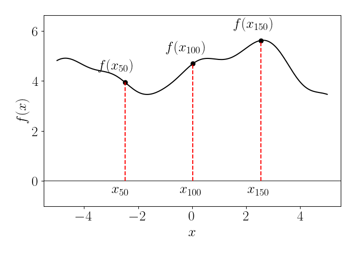
For our purposes in this post, we can think of each point (or vector) in a Hilbert space $H$ as a function. When the Hilbert space has infinite dimension, each element in the space corresponds to a vector of infinite length:
\[f = \begin{bmatrix} a_1 \\ a_2 \\ a_3 \\ \vdots \end{bmatrix}.\]While traditional vectors are indexed by the natural numbers $1, 2, 3, \dots$, we can think of each element of this vector as being indexed by a value $x$ in a domain $\mathcal{X}$. We can denote the $x$th value of the vector as $f(x)$. As you can probably tell from this notation, this is naturally leading us to think of each element of a Hilbert space as a function defined on a set $\mathcal{X}$.
We show a (unrealistic) depiction of this in the plot below. We can think of each point on this function (black line) as an element in the vector $f$. Here, I’ve labeled a few sample points in the domain with subscripts that are natural numbers $x_i, i \in \mathbb{N}$, but of course, in reality there are an infinite number of these points (where each point corresponds to a “dimension” in the Hilbert space).
A Hilbert space is then also equipped with an inner product, which in this case will be an inner product between two functions $f$ and $g$, or an inner product between two vectors of infinite length. For example, a well-studied Hilbert space is the space of all square integrable functions, whose inner product is given by
\[\langle f, g \rangle = \int_\mathcal{X} f(x) g(x) dx.\]To evaluate the function represented by a given element, a Hilbert space has an evaluation functional $L_x$ that evaluates a function $f$ at all points $x \in \mathcal{X}$. Specifically, for all functions $f \in \mathcal{H}$, the evaluation functional is defined as
\[L_x : f \mapsto f(x).\]Reproducing kernel Hilbert spaces
A reproducing kernel Hilbert space (RKHS) is a special type of Hilbert space. Technically, an RKHS is a Hilbert space whose evaluation functional is bounded and linear. However, the most practically useful characterization of an RKHS is that it’s a Hilbert space in which we can represent the evaluation functional $L_x$ as an inner product. Specifically, in an RKHS, for any function $f \in \mathcal{H}$ we have
\[f(x) = L_x(f) = \langle f, K_x \rangle_{\mathcal{H}},\]where $K_x \in \mathcal{H}$. Notice that $K_x$ is also a function defined on $\mathcal{H}$, so we can represent its evaluation at any point $y \in \mathcal{X}$ using the linear functional $L_y$ applied to $K_x$:
\[K_x(y) = L_y(K_x)\]Applying the definition of an RKHS again, we can represent this evaluation in terms of an inner product:
\[L_y(K_x) = \langle K_x, K_y \rangle_\mathcal{H},\]where $K_y \in H$ is the element in $\mathcal{H}$ satisfying the reproducing property for $y$. This finally yields the “reproducing kernel” of $H$, which is a function $K : \mathcal{X} \times \mathcal{X} \to \mathbb{R}$ satisfying
\[K(x, y) = \langle K_x \,, K_y \rangle_{\mathcal{H}}.\]In other words, we can evaluate any function in an RKHS by just using an inner product with another element in the RKHS.
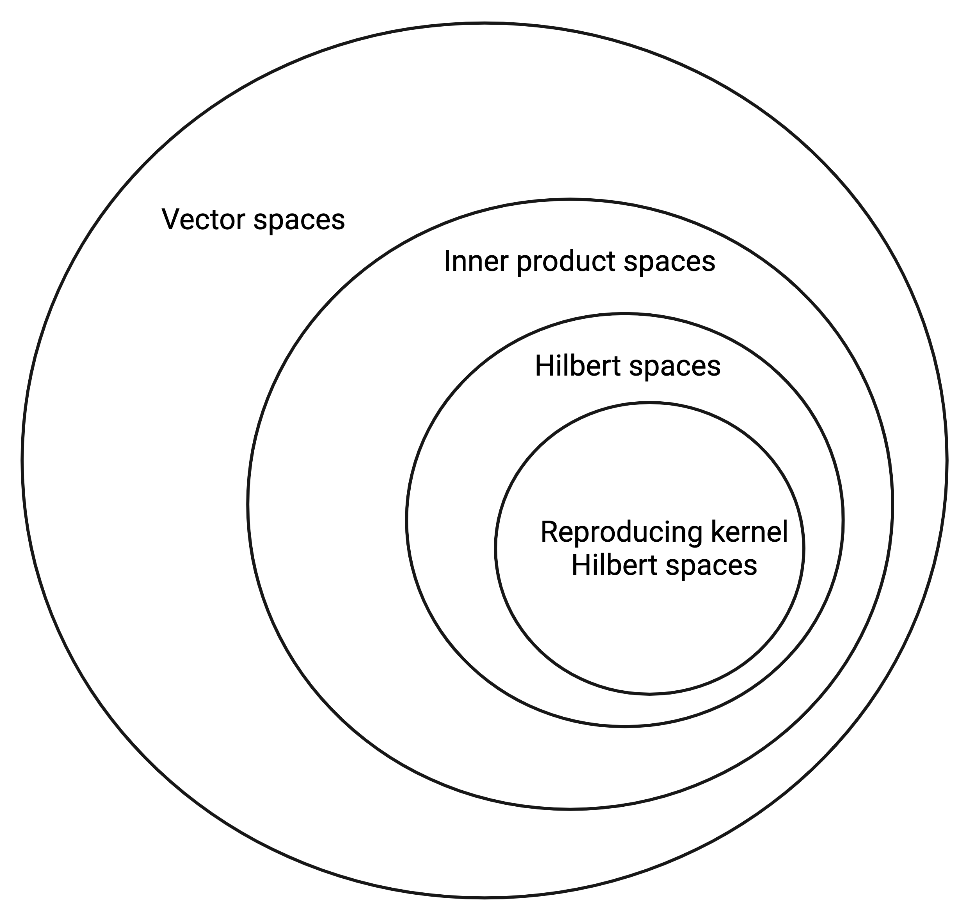
We can visualize the relationship between all of the different vector spaces mentioned above in the diagram below.
Regression
The properties of the RKHS allow for performing nonparametric regression that would seem intractable otherwise. Consider the following problem:
\[\min_{f \in \mathcal{H}} \sum\limits_{i=1}^n (y_i - f(\mathbf{x}_i))^2 + \lambda \|f\|_{\mathcal{H}}^2.\]In its current form, this optimization problem represents a minimization over an infinite number of functions. This seems wildly intractable on its face. However, the representer theorem states that the solution must have tbe following simple form:
\[f^\star(\mathbf{x}^\prime) = \sum\limits_{i=1}^n \alpha_i K(\mathbf{x}_i, \mathbf{x}^\prime),\]where $K(\cdot, \cdot)$ is the kernel associated with $\mathcal{H}$. This means that we only need to optimize over the finite coefficient vector $\boldsymbol{\alpha} = (\alpha_1, \cdots, \alpha_n)^\top$, rather than an infinite number of functions – a big improvement!
Moreover, we know that we can represent the function norm as
\[\|f\|_{\mathcal{H}}^2 = \boldsymbol{\alpha}^\top \mathbf{K} \boldsymbol{\alpha},\]where $\mathbf{K}$ is a matrix with $[\mathbf{K}]_{ij} = K(\mathbf{x}_i, \mathbf{x}_j)$. We can also denote the function evaluation at a training point as $f(\mathbf{x}_i) = \mathbf{K}_{i\cdot}^\top \boldsymbol{\alpha}$, where $\mathbf{K}_{i\cdot}$ is the $i$th row of $\mathbf{K}$. These steps simplify our optimization problem to the following:
\[\min_{\boldsymbol{\alpha} \in \mathbb{R}^n} \|\mathbf{y} - \mathbf{K} \boldsymbol{\alpha} \|^2 + \lambda \boldsymbol{\alpha}^\top \mathbf{K} \boldsymbol{\alpha}.\]We can now easily solve this with calculus. Letting $\mathcal{L}$ denote the loss function above, we can expand it as follows:
\[\mathcal{L} = \mathbf{y}^\top \mathbf{y} - 2 \boldsymbol{\alpha}^\top \mathbf{K} \mathbf{y} + \boldsymbol{\alpha}^\top \mathbf{K} \mathbf{K} \boldsymbol{\alpha} + \lambda \boldsymbol{\alpha}^\top \mathbf{K} \boldsymbol{\alpha}.\]Taking the derivative with respect to $\boldsymbol{\alpha}$, we have
\[\frac{\partial \mathcal{L}}{\partial \boldsymbol{\alpha}} = -2 \mathbf{K} \mathbf{y} + 2 \mathbf{K} \mathbf{K} \boldsymbol{\alpha} + 2 \lambda \mathbf{K} \boldsymbol{\alpha}.\]Equating this to zero and left-multiplying by $\mathbf{K}^{-1}$ leaves us with
\[\mathbf{K} \mathbf{K} \boldsymbol{\alpha} + \mathbf{K} \boldsymbol{\alpha} = \mathbf{K} \mathbf{y} \implies \mathbf{K} \boldsymbol{\alpha} + \lambda \boldsymbol{\alpha} = \mathbf{y}.\]This leads us to the following solution:
\[\boldsymbol{\alpha}^\star = (\mathbf{K} + \lambda \mathbf{I}_n)^{-1} \mathbf{y}.\]For a test point $\mathbf{x}^\prime$, the RKHS prediction is then
\[\widehat{y} = \mathbf{k}_{\mathbf{x}^\prime}^\top \boldsymbol{\alpha}^\star = k_{\mathbf{x}^\prime}^\top (\mathbf{K} + \lambda \mathbf{I}_n)^{-1} \mathbf{y},\]where $\mathbf{k}_{\mathbf{x}^\prime}$ is the vector with $[\mathbf{k}_{\mathbf{x}^\prime}]_i = K(\mathbf{x}_i, \mathbf{x}^\prime)$.
Notice that this is also the posterior mean function for a Gaussian process with covariance function $K(\cdot, \cdot)$ and noise variance $\lambda$.
References
- Sayan Mukherjee’s notes on reproducing kernel Hilbert spaces.
- Ryan Tibshirani’s notes on the topic.
- Wikipedia entries for RKHS and Hilbert spaces.