Andy Jones
The representer theorem and kernel ridge regression
The representer theorem is a powerful result that implies a certain type of duality between solutions to function estimation problems.
The Representer Theorem
To start, let’s define an informal version of the Representer Theorem that avoids some of the dirty (yet important) details. Generally, the Representer Theorem states that any function estimation problem that is formulated in terms of a loss function over the observed data, plus a regularizing term, has a solution that is a simple finite weighted sum over the data points that have been passed through a “kernel function”. In other words, we’re considering problems in which we’d like to find a function $f$ via the following optimization problem:
\[\text{arg}\min_f L(f(\textbf{X}), \textbf{Y}) + R(f)\]where $L$ is some loss function measuring how close the predictions $f(\textbf{X})$ are to the true response variables $\textbf{Y}$, and $R(f)$ is a regularization term that penalizes the complexity of the function $f$. Then, the Representer Theorem says that the minimizer $f^*$ of this problem is
\[f(\cdot) = \sum\limits_{i=1}^n \alpha_i K(\cdot, X_i)\]where $K$ is a kernel that measures the similarity between two data points. In words, this means that the optimal prediction for a new test data point can be expressed as a simple sum over observed training data points.
Of course, the intuition above has glossed over some important details, such as which types of loss functions and regularization functions are valid, where $K$ comes from, how to compute $\alpha_i$.
To state the theorem a bit more formally, consider the version from Fan et al., 2020:
Consider a general loss function $L(y, f(\textbf{x}))$, and let
\[\hat{f} = \text{arg}\min_{f \in \mathcal{H}\_K} \sum\limits_{i=1}^n L(y_i, f(\textbf{x}\_i) + R_\lambda(||f||_{\mathcal{H}_K})\]where $\mathcal{H}_K$ is a reproducing Kernel Hilbert space with kernel $K$, $\lambda > 0$, and $R_\lambda(t)$ is a srictly increasing function on $[0, \infty)$. Then we must have
\[\hat{f}(\mathbf{x}) = \sum\limits_{i=1}^n \hat{\alpha}_i K(\mathbf{x}, X_i)\]where $\hat{\boldsymbol{\alpha}} = (\hat{\alpha}_1, \dots, \hat{\alpha}_n$ is the solution to the following problem:
\[\min_{\hat{\boldsymbol{\alpha}}} \sum\limits_{i=1}^n L\left( y_i, \sum\limits_{j=1}^n \alpha_j K(\mathbf{x}, \mathbf{x}_j) \right) + R_\lambda(\sqrt{\boldsymbol{\alpha} \mathbf{K} \boldsymbol{\alpha}}).\]Kernel ridge regression
To make things a bit more concrete, let’s consider the simplest example/application of the Representer Theorem. Suppose we choose the following for a specific problem:
- Loss function is $L(y_i, f(\textbf{x}_i)) = (y_i - f(\textbf{x}_i))^2$
- Regularization function is $R_\lambda(||f||_{\mathcal{H}_K}) = \lambda ||f||_{\mathcal{H}_K}^2$
- Kernel function is the linear kernel $K(\textbf{x}_i, \textbf{x}_j) = \textbf{x}_i^\top \textbf{x}_j$. Then the optimization problem becomes:
and the solution for $\boldsymbol{\alpha}$ becomes
\[\min_{\hat{\boldsymbol{\alpha}}} ||\textbf{Y} - \textbf{K}\boldsymbol{\alpha}||^2 + \lambda \boldsymbol{\alpha}^\top \textbf{K} \boldsymbol{\alpha}.\]Taking the gradient with respect to $\boldsymbol{\alpha}$ and setting it to zero, we have
\[-\textbf{K}\textbf{Y} + \textbf{K}\textbf{K} \alpha + \lambda \textbf{K} \alpha = 0.\]Rearranging, we have
\begin{align} \textbf{K}\textbf{K} \boldsymbol{\alpha} + \lambda \textbf{K} \boldsymbol{\alpha} &= \textbf{K} y \\ \boldsymbol{\alpha} (\textbf{K} \textbf{K} + \lambda \textbf{K}) &= \textbf{K} \textbf{Y} \\ \boldsymbol{\alpha} &= (\textbf{K} \textbf{K} + \lambda \textbf{K})^{-1} \textbf{K} \textbf{Y} \\ \boldsymbol{\alpha} &= (\textbf{K} + \lambda \textbf{I}_n)^{-1} \textbf{K}^{-1} \textbf{K} \textbf{Y} \\ \boldsymbol{\alpha} &= (\textbf{K} + \lambda \textbf{I}_n)^{-1} \textbf{Y} \\ \end{align}
Notice that this expression only requires us to evaluate the inner product (or more generally, the kernel function) between all pairs of data points. So regardless of how many covariates there are (and there could be many), we never have to sum over that dimension.
In contrast, recall the usual estimator for ridge regression:
\[\hat{\beta} = (\textbf{X}^\top \textbf{X} + \lambda \mathbf{I}_p) \textbf{X}^\top \textbf{Y}.\]It turns out that, not only is ridge regression solving the same problem, but there’s also a one-to-one correspondence between the solution for $\alpha$ is kernel ridge regresion and the solution for $\beta$ in ridge regression. However, there’s a key difference in how they’re computed. Notice that to find $\beta$, we must sum over the dimension of the covariates, which is $p$, while in kernel ridge regression we only had to sum over the number of data points, $n$. As we’ll see below, each of these has computational tradeoffs depending on the model and dataset.
Timing kernel ridge regression
To demonstrate the computational benefits of kernel ridge regression, we can compare the time required to estimate $\boldsymbol{\alpha}$ and $\boldsymbol{\beta}$ for kernel ridge and ridge regression, respectively, as the number of covariates $p$ increases. Remember, because ridge regression requires a sum over $n$ and kernel regression requires a sum over $p$, we expect kernel ridge regression to be faster as $p$ becomes very large.
The following code runs this experiment for varying values of $p$:
import time
import numpy as np

n = 500
lam = 10
p_seq = np.arange(10, 2001, step=100)

ridge_times = []
kernel_ridge_times = []
for ii, p in enumerate(p_seq):

    # Generate data and true model
    X = np.random.normal(loc=0, scale=1, size=(n, p))
    beta = np.random.normal(loc=0, scale=1, size=p)
    epsilon = np.random.normal(loc=0, scale=1, size=n)
    Y = np.matmul(X, beta) + epsilon

    # Ridge regression
    start = time.time()
    XTX_inv = np.linalg.inv(np.matmul(X.T, X) + lam*np.eye(p))
    XTY = np.matmul(X.T, Y)
    beta_hat_ridge = np.matmul(XTX_inv, XTY)
    end = time.time()
    ridge_times.append(end - start)

    # Kernel ridge regression
    start = time.time()
    XXT_inv = np.linalg.inv(np.matmul(X, X.T) + lam*np.eye(n))
    XTK_inv = np.matmul(X.T, XXT_inv)
    beta_hat_kernel_ridge = np.matmul(XTK_inv, Y)
    end = time.time()
    kernel_ridge_times.append(end - start)
And here are the results:
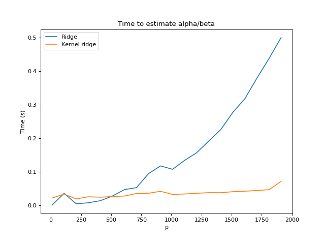
As we expected, with an increasing value of $p$, ridge regression requires more and more time to compute the estimated coefficients. On the other hand, kernel ridge regression remains fairly constant. Also, notice that we used a value of $n = 500$, and the two methods cross paths very close to $p = 500$, since for a square matrix $\mathbf{X} \in \mathbb{R}^{n\times p}$ where $n=p$, the two methods require the same number of operations.
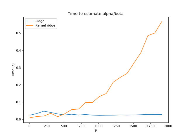
We can also do the reverse experiment, with increasing $n$, and we obtain the opposite results — kernel ridge regression scales poorly, while ridge regression requires about constant time:
Conclusion
Here, we reviewed the Representer Theorem and some of its implications for estimating nonparametric functions. We also saw that it has practical implications for reducing compute time by avoiding computation over large feature spaces.
References
- Fan, J., Li, R., Zhang, C.-H., and Zou, H. (2020). Statistical Foundations of Data Science. CRC Press, forthcoming.
- Prof. Martin Wainwright’s lecture notes
- Emtiyaz Khan’s notes