RBF kernel as an infinite feature expansion

The radial basis function (RBF) kernel is one of the most commonly-used kernels in kernel methods. Here, we show how the kernel arises from taking an infinite polynomial feature expansion. We show this in the setting of linear regression.

Recall the RBF kernel (AKA squared exponential, exponentiated quadratic, Gaussian, …),

We can recover this kernel by considering a linear model with infinite feature expansions. In particular, consider the linear function

where $\phi: \mathbb{R} \mapsto \mathbb{R}^q$ is a function that maps our features to a higher-dimensional space. Notice that the covariance of this function has the following form:

\begin{align} cov(f(x_i), f(x_j)) &= \mathbb{E}[(w^\top \phi(x_i))^\top (w^\top \phi(x_j))] \\ &= \mathbb{E}[\phi(x_i)^\top ww^\top \phi(x_j)] \\ &= \phi(x_i)^\top \mathbb{E}[ww^\top] \phi(x_j) \\ &= \sigma^2 \phi(x_i)^\top \phi(x_j). \\ \end{align}

Consider the following form for $\phi$,

where $\phi(x)_k$ denotes the $k$th element of $\phi(x)$. Notice that this is essentially a polynomial feature expansion,

but scaled by a constant term.

Plugging this into our covariance above, we have

\begin{align} cov(f(x_i), f(x_j)) &= \sigma^2 \phi(x_i)^\top \phi(x_j) \\ &= \sigma^2 \exp\{-\frac{1}{2\ell^2} x_i^2\} \exp\{-\frac{1}{2\ell^2} x_j^2\} \sum\limits_{k=0}^q \frac{(x_i)^k}{\ell^k \sqrt{k!}} \cdot \frac{(x_j)^k}{\ell^k\sqrt{k!}} \\ &= \sigma^2 \exp\{-\frac{1}{2\ell^2} (x_i^2 + x_j^2)\} \sum\limits_{k=0}^q \frac{(x_i x_j)^k}{\ell^{2k} k!} \\ &= \sigma^2 \exp\{-\frac{1}{2\ell^2} (x_i^2 + x_j^2)\} \sum\limits_{k=0}^q \left(\frac{x_i x_j}{\ell^2}\right)^k \frac{1}{k!}. \\ \end{align}

If we let $q\to\infty$, then we can recognize the sum as the Taylor expansion of $\exp\left\{\frac{x_i x_j}{\ell^2}\right\}$. We then have

\begin{align} cov(f(x_i), f(x_j)) &= \sigma^2 \exp\{-\frac{1}{2\ell^2} (x_i^2 + x_j^2)\} \exp\{\frac{1}{\ell^2} x_i x_j\} \\ &= \sigma^2 \exp\{-\frac{1}{2\ell^2} (x_i^2 + x_j^2 - 2x_ix_j)\} \\ &= \sigma^2 \exp\{-\frac{1}{2\ell^2} (x_i - x_j)^2\} \\ \end{align}

Thus, we can see that the kernel arises from a feature expansion of infinite polynomials. Notice that the $\sigma^2$ paramters is determined by our prior variance on the linear model weights $w$, and the length scale parameter $\ell$ is determined by our chosen constant in the feature expansion.

Visualization

One way to visualize kernels is to plot heatmaps of the kernel’s values over a grid of space. Below, I show a simple example using just a finite sum of the polynomial features above. In other words, I just truncate the sum up to a finite $q$. Here, I take $q \in \{1, 2, 3, 10\}$ for demonstration.

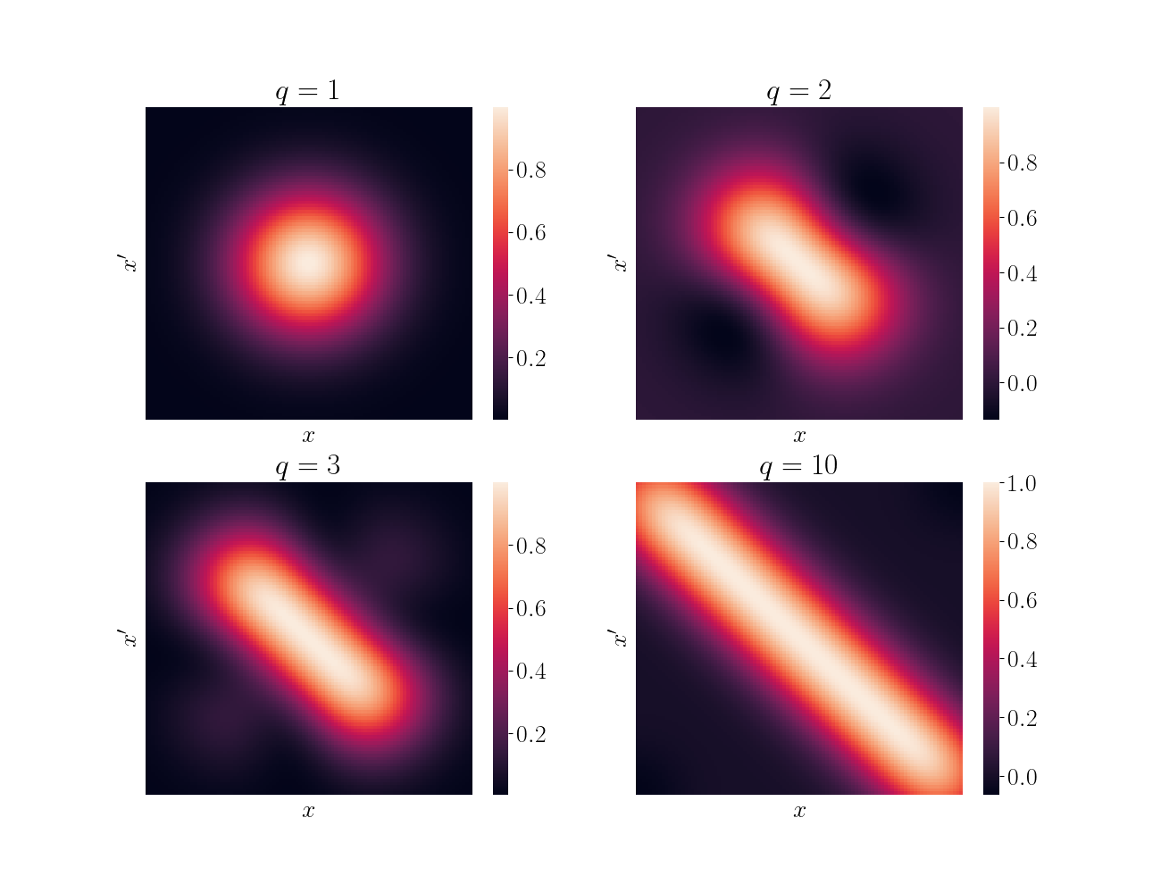
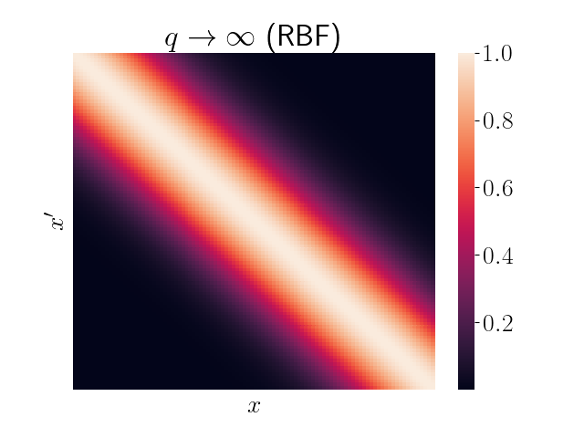
We can see that as $q$ increases, the kernel more closely resembles the true limiting kernel. Below is the analogous heatmap using the full RBF kernel.

Code

The code for the visualization above can be found below.

import numpy as np
import pandas as pd
import matplotlib.pyplot as plt
import seaborn as sns

import matplotlib
font = {"size": 20}
matplotlib.rc("font", **font)
matplotlib.rcParams["text.usetex"] = True

def finite_rbf(x, y, q, sigma2=1, length_scale=1):

	# Constant term
	C = sigma2 * np.exp(-0.5 * length_scale**2 * (x**2 + y**2))

	# Interaction between x, y
	qsum = 0
	for k in range(q):
		curr_summand = (x * y / length_scale**2)**k * 1 / (np.math.factorial(k))
		qsum += curr_summand

	return C * qsum


def getK(x, q):
	K = np.zeros((n, n))
	for ii in range(len(x)):
		for jj in range(ii + 1):
			curr_k = finite_rbf(x[ii], x[jj], q=q)
			K[ii, jj] = curr_k
			K[jj, ii] = curr_k

	assert np.all(K == K.T)
	return K

n = 100
x = np.linspace(-3, 3, n)

qs = [1, 2, 3, 10]

plt.figure(figsize=(13, 10))
for ii, q in enumerate(qs):
	plt.subplot(2, 2, ii + 1)
	K = getK(x, q=q)
	sns.heatmap(K)
	plt.xticks([])
	plt.yticks([])
	plt.xlabel(r"$x$")
	plt.ylabel(r"$x^\prime$")
	plt.title(r"$q={}$".format(q))
plt.savefig("./out/finite_rbf.png")
plt.show()

References

• Matthew N. Bernstein’s notes on the RBF kernel.
• Yaser Abu-Mostafa’s lecture video on kernel methods.