Rayleigh distribution (aka polar transformation of Gaussians)

In this post, we’ll look at a simple example of performing transformations on random variables. Specifically, we’ll explore what happens when two independent Gaussian-distributed random variables are transformed to polar coordinates.

Setup

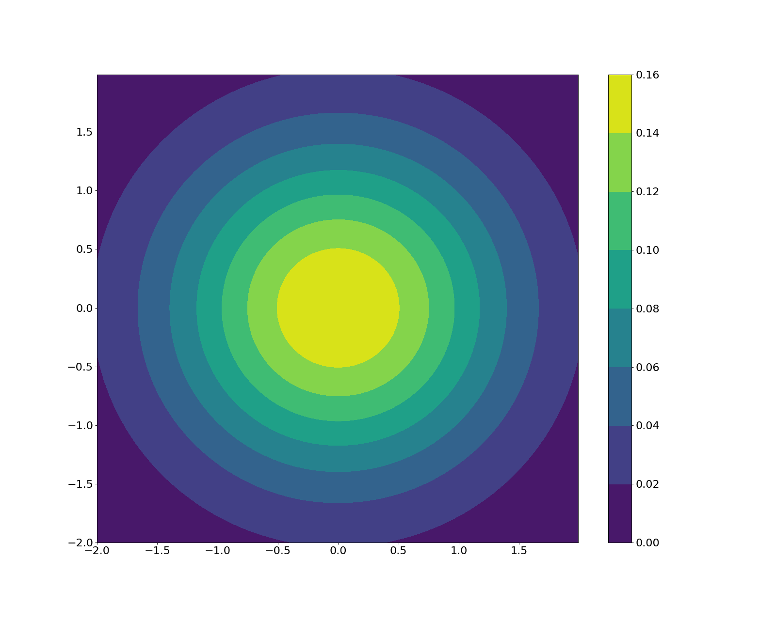
Consider two random variables $X$ and $Y$ that are independent and identically distributed from a zero-mean Gaussian with variance of $1$.

\[X, Y \stackrel{iid}{\sim} \mathcal{N}(0, 1)\]

We can easily visualize their joint distribution:

Now, consider the transformation to two new random variables $R$, $\Theta$ such that

\[R = \sqrt{X^2 + Y^2}\] \[\Theta = \tan^{-1}\big(\frac{Y}{X}\big)\]

Also recall that we can transform from $R$ and $\Theta$ to $X$ and $Y$ by the following relationship:

\[X = r \cos \theta \quad \textrm{and} \quad Y = r \sin \theta.\]

Computing the transformation

Now, in order to compute the joint and marginal distributions of $R$ and $\Theta$, we can use the Jacobian transformation technique. Recall that the Jacobian transformation method defines the relationship between sets of random variables that have a one-to-one mapping between them. In our case, since we know the densities of $X$ and $Y$, we can write the joint density of $R$ and $\Theta$ as

\[f_{R, \Theta}(r, \theta) = f_{X, Y}(g_1^{-1}(r), g_2^{-1}(\theta))|J|\]

where $g_1^{-1}(r) = r \cos \theta$, $g_2^{-1}(\theta) = r \sin \theta$, and $\lvert J\rvert$ is the Jacobian of the transformation. That is:

\begin{align}\lvert J\rvert &= \begin{vmatrix} \frac{\delta x}{\delta r} & \frac{\delta y}{\delta r} \\ \frac{\delta x}{\delta \theta} & \frac{\delta y}{\delta \theta} \end{vmatrix}\end{align}

First, let’s compute the Jacobian of the transformation:

\begin{align}\det J &= \begin{vmatrix} \frac{\delta x}{\delta r} & \frac{\delta y}{\delta r} \\ \frac{\delta x}{\delta \theta} & \frac{\delta y}{\delta \theta} \end{vmatrix} \\ &= \begin{vmatrix} \cos \theta & \sin \theta \\ -r\sin\theta & r\cos\theta \end{vmatrix} \\ &= r\cos^2\theta + r\sin^2\theta \\ &= r \end{align}

Also, because $X$ and $Y$ are independent, we can simply multiply their individual densities to get their joint density:

\[f_{X, Y}(x, y) = \frac{1}{2\pi} e^{-\frac{x^2 + y^2}{2}}.\]

Writing out the full density of $R$ and $\Theta$, we have

\begin{align}f_{R, \Theta}(r, \theta) &= f_{X, Y}(g_1^{-1}(r), g_2^{-1}(\theta))\lvert J\rvert \\ &= \frac{1}{2\pi} e^{-\frac{r^2\cos^2\theta * r^2\sin^2\theta}{2}}r \\ &= \frac{1}{2\pi} e^{\frac{r^2}{2}}r\end{align}

where the $r$ at the end comes from the Jacobian computed above. Notice that $\theta$ doesn’t appear in this joint distribution, meaning that it’s constant in $\theta$, and $\theta$ is uniformly distributed.

To compute the marginal distributions for $R$ and $\Theta$, we can integrate out $\Theta$ and $R$, respectively.

\[f_R(r) = \int_0^{2\pi} f_{R, \Theta}(r, \theta) d\theta = re^{-\frac{r^2}{2}}\] \[f_\Theta(\theta) = \int_0^{\infty} f_{R, \Theta}(r, \theta) dr = \frac{1}{2\pi}\]

Notice that $f_{R, \Theta}(r, \theta) = f_R(r)f_\Theta(\theta)$, indicating that $R$ and $\Theta$ are independent.

The distribution $f_R(r)$ above is known as a Rayleigh distribution, a common density whose practical usefulness is discussed later. It’s a special case of the chi distribution, and also has close ties to the chi-squared and gamma distributions.

Simulations

Taking a step back, let’s see what this means. We started with two Gaussian-distributed random variables $X$ and $Y$. One way to think about a sample from $X$ and $Y$ is as a vector in $\mathbb{R}^2$ (i.e. draw an x-value, draw a y-value, and the $(x, y)$ pair will be the vector). Then, by computing the distributions of two transformations $R$ and $\Theta$, we were essentially computing the distribution of the lengths and angles of the vectors drawn from the 2D Gaussian, respectively.

Let’s take a look at the distribution of $R$:

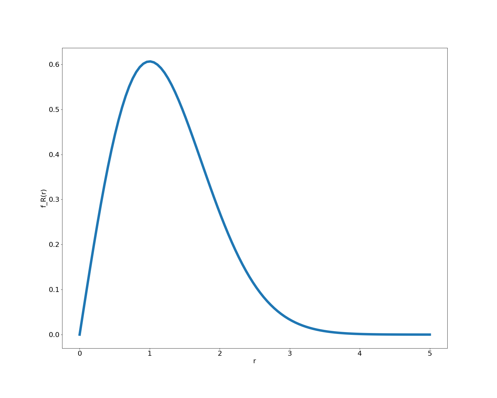
Loosely speaking, its shape implies that most of the vectors drawn from $X, Y$ will have length around $1$.

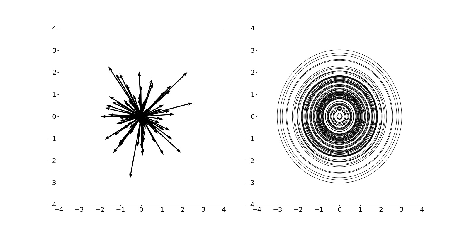
Let’s run a simple simulation to verify this. We start by drawing samples using the following procedure:

1. Draw $x$ and $y$ from $\mathcal{N}(0, 1)$ independently.
2. Compute $r = \sqrt{x^2 + y^2}$.

We can visualize these samples in vector form (left) and as a collection of concentric circles whose radii are equal to to length of the vector (right):

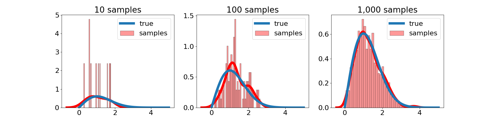
Now, let’s look at the distribution of these samples more directly. Below, we show a histogram of the $r$ samples for a varying number of samples. We also show the theoretical distribution as derived above. As expected, as more samples are drawn, the empirical distribution approaches the theoretical one.

Applications of the Rayleigh distribution

The Rayleigh distribution is useful for modeling lots of interesting processes. For example, imagine a wireless signal propagating through midtown Manhattan. On its path, the signal will hit lots of different solid objects (buildings, cars, etc.) that will change its direction and magnitude. Then the final path of the signal is just a sum of all of these direction changes. If there are enough of these barriers (as in Manhattan), the central limit theorem will kick in, and it becomes reasonable to model each direction ($x$ and $y$) as an independent Gaussian. Thus, the results we computed above would hold, and the final amplitude of the signal will be Rayleigh-distributed.

Conclusion

We worked through a simple example of transforming random variables, which resulted in the Rayleigh distribution.

References

1. Although this example can be found in many places, I learned of it from Professor Krishna Jagannathan’s online lectures for his course Probability Foundation for Electrical Engineers. I closely follow his example.
2. I also used the Wikipedia entry for the Rayleigh disribution.