Andy Jones
Quasi-likelihoods
As their name suggests, “quasi-likelihoods” are quantities that aren’t formally likelihood functions, but can be used as replacements for formal likelihoods in more general settings.
A major reason that quasi-likelihoods are useful is that they don’t require the statistician to specify a full probability distribution for the data – instead, only the first and second moments must be specified. This allows the modeler to have more flexibility without having to impose unnecessary (and incorrect) assumptions.
Most results for quasi-likelihoods are in the context of the exponential family, which we review here first.
Exponential family
Recall the form of the exponential family of distributions:
\[f(y; \theta) = \exp\left\{ a(y) b(\theta) + c(\theta) + d(y) \right\}.\]for some functions $a$, $b$, $c$, and $d$. In canonical form, we have $a(y) = y$ and $b(\theta) = \theta$. The form of the likelihood then simplifies to
\[f(y; \theta) = \exp\left\{ \frac{y \theta - b(\theta)}{a(\phi)} + c(y, \phi) \right\}\]where we call $\phi$ a “dispersion parameter”.
Likelihood for GLMs
Generalized linear models (GLMs) extend the classical linear model to allow for various types of response distributions. For a response vector $\mathbf{Y}$, a matrix of covariates $\mathbf{X}$, and a vector of coefficients $\boldsymbol{\beta}$, a GLM has the model structure of
\[\mathbb{E}[\mathbf{Y} | \mathbf{X}] = \mu(\mathbf{X}) = g^{-1}(\mathbf{X} \boldsymbol{\beta})\]where $g(\cdot)$ is a link function. Equivalently, we have $g(\mu(\mathbf{X})) = \mathbf{X}\boldsymbol{\beta}$, which we typically define to be the parameter $\theta$: $\theta = g(\mu(\mathbf{X})) = g(\mu)$. We also define $\eta$ to be the linear predictor: $\eta = \mathbf{X} \boldsymbol{\beta}$.
Additionally, $\mathbf{Y} | \mathbf{X}$ is typically assumed to come from an exponential family distribution. For a sample of size $n$, the likelihood is then
\[L(\theta) = \prod\limits_{i=1}^n \exp\left\{ \frac{y_i \theta_i - b(\theta_i)}{a(\phi)} + c(y_i, \phi) \right\}.\]The corresponding log-likelihood is
\[\ell(\theta) = \sum\limits_{i=1}^n \left[\frac{y_i \theta_i - b(\theta_i)}{a(\phi)} + c(y_i, \phi)\right].\]To perform maximum likelihood estimation, we take the derivative w.r.t. the coefficients $\beta_1, \dots, \beta_p$ and set these expressions to zero. This can be accomplished with the chain rule:
\[\frac{\partial \ell_i}{\partial \beta_j} = \frac{\partial \ell_i}{\partial \theta_i} \cdot \frac{\partial \theta_i}{\partial \mu_i} \cdot \frac{\partial \mu_i}{\partial \eta_i} \cdot \frac{\partial \eta_i}{\partial \beta_j}.\]Breaking these partial derivatives down, we have
\begin{align} \frac{\partial \ell_i}{\partial \theta_i} &= \frac{y_i - b’(\theta_i)}{a(\phi)} = \frac{y_i - \mu_i}{a(\phi)} \\ \frac{\partial \theta_i}{\partial \mu_i} &= g’(\mu_i) = (b’‘(y_i))^{-1} = \frac{a(\phi)}{\text{Var}(y_i)} = \frac{1}{v(y_i)} \\ \frac{\partial \eta_i}{\partial \beta_j} &= X_{ij} \\ \end{align}
The expression for $\frac{\partial \ell_i}{\partial \theta_i}$ follows because $b’(\theta)$ is equal to the mean $\mu$ in the exponential family (see here for an explanation). We won’t specify $\frac{\partial \mu_i}{\partial \eta_j}$ further, just to allow for an arbitrary relationship between $\mu$ and $\eta$.
Putting these together, we have
\begin{align} \frac{\partial \ell_i}{\partial \beta_j} &= \frac{y_i - \mu_i}{a(\phi)} \cdot \frac{1}{v(y_i)} \cdot \frac{\partial \mu_i}{\partial \eta_j} \cdot X_{ij} \\ &= \frac{(y_i - \mu_i) X_{ij}}{a(\phi) v(\mu_i)} \cdot \frac{\partial \mu_i}{\partial \eta_j} \end{align}
Setting these equations to zero gives us the score equations needed to perform MLE:
\[\sum\limits_{i=1}^n \frac{(y_i - \mu_i) X_{ij}}{a(\phi) v(\mu_i)} \cdot \frac{\partial \mu_i}{\partial \eta_j} = 0, \;\;\; j = 1, \dots, p\]Notice that these equations depend on the specified probability distribution through $\mu_i$ and the variance function $v(\mu)$. Specifically, once a distribution is specified, this variance function is automatically specified as well.
We now turn to quasi-likelihoods, which allow us to avoid specifying an entire distribution. Instead, we directly specify the mean-variance relationship.
Quasi-likelihoods
A quasi-likelihood is defined as
\[\int_y^\mu \frac{y - t}{a(\phi) V(t)} dt\]where $V$ is a function that relates the variance to the mean, and $a(\phi)$ is a (unknown) dispersion parameter. Differentiating, we have
\[\frac{\partial Q}{\partial \mu} = \frac{y - \mu}{a(\phi) V(\mu)}\]We can see already that this expression is equivalent to the typical likelihood case, $\frac{\partial \ell}{\partial \mu}$.
To get the full “quasi-score equations”, we have to perform one more step of the chain rule, by multiplying by $\frac{\partial \mu}{\partial \beta}$:
\[\sum\limits_{i=1}^n \frac{(y_i - \mu_i)}{a(\phi) v(\mu_i)} \cdot \frac{\partial \mu_i}{\partial \beta_j} = 0, \;\;\; j = 1, \dots, p\]Notice that the coefficient estimates $\hat{\beta}$ are the same for the full GLM case and for quasi-likelihoods. However, they will have different variance estimates.
Quasi-likelihoods corresponding to well-known likelihoods
To build intuition, it’s useful to note that many well-known distributions correspond to a particular choice of the mean-variance relationship in the world of quasi-likelihood world. The converse is not true: there are many quasi-likelihood specifications that do not map onto any known distributions.
Table 9.1 from Peter McCullagh’s book Generalized Linear Models shows several such examples:
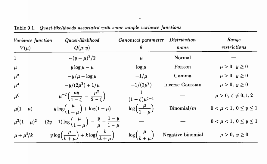
The column $Q(\mu; y)$ here is calculated by computing the integral
\[\int_y^\mu \frac{y - t}{a(\phi) V(t)} dt\]for the specified function $V(\mu)$, and it is assumed $a(\phi) = 1$ for simplicity.
For example, in the Gaussian case we have $V(\mu) = 1$, which implies
\begin{align} \int_y^\mu \frac{y - t}{a(\phi) V(t)} dt &= \int_y^\mu \frac{y - t}{1 \cdot 1} dt \\ &= \int_y^\mu (y - t) dt \\ &= -\frac12 (y - t)^2 \big\rvert_y^\mu \\ &= -\frac12 (y - \mu)^2 \end{align}
In the Poisson case, we have $V(\mu) = \mu$, which implies
\begin{align} \int_y^\mu \frac{y - t}{a(\phi) V(t)} dt &= \int_y^\mu \frac{y - t}{1 \cdot t} dt \\ &= \int_y^\mu \left(\frac{y}{t} - 1\right) dt \\ &= y \log \mu - \mu \\ \end{align}
However, notice that the table also includes variance function with no corresponding closed-form likelihood. An interesting case of this is when $V(\mu) = \mu^\zeta$, where $\zeta \neq 0, 1, 2$. This power law mean-variance relationship occurs often in ecology through Taylor’s law, and more generally in statistics it appears in the family of distributions known as the Tweedie distribution.
References
- McCullagh, Peter. Generalized linear models. Routledge, 2018.
- Agresti, Alan. Foundations of linear and generalized linear models. John Wiley & Sons, 2015.
- Islam, M. Ataharul, and Rafiqul I. Chowdhury. Analysis of repeated measures data. Singapore: Springer, 2017.