Estimation and Inference in probabilistic models: A whirlwind tour

Probabilistic models are flexible tools for understanding a data generating process. There are many ways to do inference and estimation in these models, and it continues to be an active area of research. Here, our goal will be to understand a few of the most general classes of probabilistic model fitting, while trying to understand the important differences between them. We’ll demonstrate how to implement each one with a very simple example: the Beta-Bernoulli model.

Setup

Consider the following model for some data we observe $X_1, \dots, X_n \in {0, 1}$.

\begin{align} X_i &\sim \text{Bernoulli}(\rho), \;\; i = 1, \dots, n \\ \rho &\sim \text{Beta}(\alpha, \beta) \\ \end{align}

This is one of the simplest possible probabilistic models: each of the $X_i$ is drawn from a Bernoulli distribution with parameter $\rho$, and $\rho$ in turn is drawn from a Beta distribution with parameters $\alpha$ and $\beta$. We’ll treat $\rho$ as a parameter we’d like to estimate, and $\alpha$ and $\beta$ as hyperparameters which we’ll fix to some values beforehand. The simplicity of this model will make it easier to understand each estimation and inference method, as well as the trade-offs between them.

Recall that the PDFs for the Bernoulli and Beta distributions are

and

where $B(\cdot, \cdot)$ is the Beta function

and $\Gamma$ is the Gamma function. Note that an alternative definition of the Beta function is

Full Bayesian inference

In full Bayesian inference, we seek to estimate the full posterior of the parameters given the data. In our case, since we have just one parameter, we want to estimate $p(\rho | X)$. By Bayes rule, we have

\begin{align} p(\rho | X) &= \frac{p(X | \rho) p(\rho)}{p(X)} \\ &= \frac{p(X | \rho) p(\rho)}{\int_0^1 p(X | \rho) p(\rho) d\rho}. \\ \end{align}

We already know how to express $p(X | \rho)$ and $p(\rho)$ from above (the Bernoulli and Beta density functions, respectively). However, it’s less obvious how to express the integral in the denominator in a nicer way.

Let’s write the integral out and see what pops out. Again suppose we have $n$ data points $X_1, \dots, X_n$.

\begin{align} \int_0^1 p(X_1, \dots, X_n | \rho) p(\rho) d\rho &= \int_0^1 \prod\limits_{i=1}^n \left[ \rho^{X_i} (1-\rho)^{1-X_i} \right] \frac{\rho^{\alpha - 1} (1-\rho)^{\beta - 1}}{B(\alpha, \beta)} d\rho \\ &= \int_0^1 \rho^{\sum\limits_{i=1}^n X_i} (1-\rho)^{\sum\limits_{i=1}^n (1-X_i)} \frac{\rho^{\alpha - 1} (1-\rho)^{\beta - 1}}{B(\alpha, \beta)} d\rho \\ &= \int_0^1 \rho^{\alpha - 1 + \sum\limits_{i=1}^n X_i} (1-\rho)^{\beta - 1 + \sum\limits_{i=1}^n (1-X_i)} \frac{1}{B(\alpha, \beta)} d\rho \\ &= \frac{1}{B(\alpha, \beta)} \int_0^1 \rho^{\alpha - 1 + \sum\limits_{i=1}^n X_i} (1-\rho)^{\beta - 1 + \sum\limits_{i=1}^n (1-X_i)} d\rho \\ &= \frac{1}{B(\alpha, \beta)} B\left(\alpha + \sum\limits_{i=1}^n X_i, \beta + \sum\limits_{i=1}^n (1-X_i)\right) \\ \end{align}

where the last equality follows from the second definition of the Beta function that we gave above.

Putting these together, we have that the posterior distribution is

\begin{align} p(\rho | X) &= \frac{p(X | \rho) p(\rho)}{\int_0^1 p(X | \rho) p(\rho) d\rho} \\ &= \frac{\rho^{\sum\limits_{i=1}^n X_i} (1-\rho)^{\sum\limits_{i=1}^n (1-X_i)} \frac{\rho^{\alpha - 1} (1-\rho)^{\beta - 1}}{B(\alpha, \beta)}}{\frac{1}{B(\alpha, \beta)} B\left(\alpha + \sum\limits_{i=1}^n X_i, \beta + \sum\limits_{i=1}^n (1-X_i)\right)} \\ &= \frac{\rho^{\sum\limits_{i=1}^n X_i} (1-\rho)^{\sum\limits_{i=1}^n (1-X_i)} \rho^{\alpha - 1} (1-\rho)^{\beta - 1}}{B \left(\alpha + \sum\limits_{i=1}^n X_i, \beta + \sum\limits_{i=1}^n (1-X_i)\right)} \\ &= \frac{\rho^{\alpha - 1 + \sum\limits_{i=1}^n X_i} (1-\rho)^{\beta - 1 + \sum\limits_{i=1}^n (1-X_i)}}{B \left(\alpha + \sum\limits_{i=1}^n X_i, \beta + \sum\limits_{i=1}^n (1-X_i)\right)} \\ \end{align}

The last line is the PDF of the beta distribution with parameters $\alpha^* = \alpha + \sum\limits_{i=1}^n X_i$ and $\beta^* = \beta + \sum\limits_{i=1}^n (1-X_i)$. So we started with a Beta prior on $\rho$, and after seeing some data, we have another Beta distribution for $\rho$, but it has been updated. This type of prior — where the prior has the same distribution as the likelihood — is called a conjugate prior. In this case, the Beta distribution is a conjugate prior for the Bernoulli distribution.

Notice that in this case, the integral in the denominator of the posterior,

could be solved analytically and had a very nice form. This will not be true in general, and the general intractability of this integral is the motivation for many other methods of fitting probabilistic models.

Let’s see how to implement this in Python (it just amounts to adding new values to $\alpha$ and $\beta$.

import numpy as np
import matplotlib.pyplot as plt
from scipy.stats import beta

n = 20
p = 0.2
X = np.random.binomial(n=1, p=p, size=n)

a = 0.5
b = 0.5

## Full Bayesian
anew = a + np.sum(X)
bnew = b + np.sum(1 - X)

Here, we set $\alpha = \beta = 0.5$, which puts more weight on values of $\rho$ that are closer to the edges of its support: near $0$ or $1$.

We can then plot the prior and posterior, with the true value of $\rho$ shown as a dotten red line on the right:

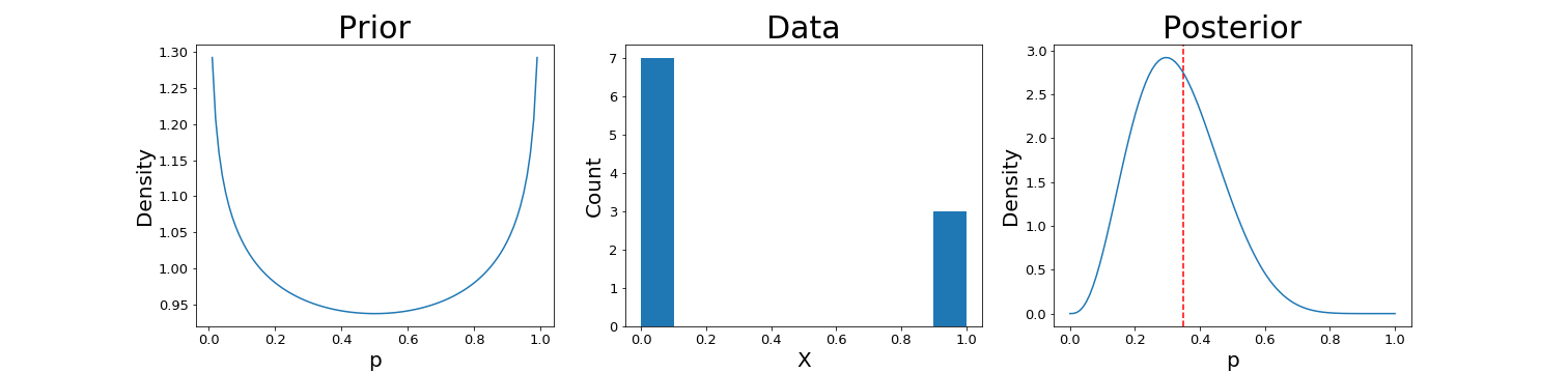
It’s worth playing with the hyperparameters $\alpha$ and $\beta$ (as well as the size of the dataset $n$) to see how their values affect the outcome.

Maximum likelihood estimation

Maximum likelihood estimation (MLE) is a family of estimation procedures that seeks the parameter value(s) that maximize the likelihood of having observed the data at hand. In our Beta-Bernoulli case, this means that we effectively ignore the prior, and focus on maximizing $p(X | \rho)$.

Recall that this Bernoulli likelihood for $n$ data points is given as

\begin{align} p(X | \rho) &= \prod\limits_{i=1}^n \left[ \rho^{X_i} (1-\rho)^{1-X_i} \right] \\ &= \rho^{\sum\limits_{i=1}^n X_i} (1-\rho)^{\sum\limits_{i=1}^n 1-X_i} \\ \end{align}

It’s often easier to maximize the log-likelihood:

\begin{align} \log p(X | \rho) &= \left[\sum\limits_{i=1}^n X_i \right] \log \rho + \left[\sum\limits_{i=1}^n 1-X_i \right] \log (1-\rho) \\ &= \left[\sum\limits_{i=1}^n X_i \right] \log \rho + \left[n - \sum\limits_{i=1}^n X_i \right] \log (1-\rho) \\ \end{align}

We can then differentiate with respect to $\rho$, set to $0$, and solve:

\begin{align} &\frac{d}{d \rho} \log p(X | \rho) = \frac1\rho \sum\limits_{i=1}^n X_i - \frac{1}{1-\rho} \left[n - \sum\limits_{i=1}^n X_i \right] = 0 \\ \implies& \frac1\rho \sum\limits_{i=1}^n X_i = \frac{1}{1-\rho} \left[n - \sum\limits_{i=1}^n X_i \right] \\ \implies& (1 - \rho) \sum\limits_{i=1}^n X_i = \rho \left[n - \sum\limits_{i=1}^n X_i \right] \\ \implies& \sum\limits_{i=1}^n X_i - \rho \sum\limits_{i=1}^n X_i = \rho n - \rho \sum\limits_{i=1}^n X_i \\ \implies& \hat{\rho}_{\text{MLE}} = \frac1n \sum\limits_{i=1}^n X_i \\ \end{align}

Thus, the maximum likelihood estimate for the Bernoulli model is simply the sample average.

In general, if the MLE isn’t available in closed form, we can also estimate it using iterative methods like gradient ascent, as shown for the Bernoulli model in Python below.

## Maximum likelihood
# max p(x | theta)
#
# LL = sum(x) * log(p) + sum(1-x) * log(1-p)

def LL(x, p):
    return np.sum(x) * np.log(p) + np.sum(1 - x) * np.log(1 - p)

# Derivative wrt p
def LL_grad(x, p):
    return (np.sum(x) / p - np.sum(1 - x) / (1 - p)) / n

curr_p = 0.1
for _ in range(100):
    curr_p += LL_grad(X, curr_p) * 0.01
    
print("MLE estimate: {}".format(round(curr_p, 4)))

Maximum a posteriori (MAP) estimation

Another family estimation procedures that provides a point estimate is called maximum a posteriori (MAP) estimation. In MAP estimation, we also incorporate the prior into the point estimate. In particular, we find the parameter value(s) that maximize the posterior $p(\rho | X)$. Recall that, using Bayes rule, we can rewrite the posterior as

Notice that the denominator, $\int_0^1 p(X | \rho) p(\rho) d\rho = p(X)$ will not depend on $\rho$, and is thus constant for the purposes of maximizing w.r.t $\rho$. Thus, in MAP we seek to maximize the numerator only, which will always be proportional to the posterior:

Writing this out, we have

Similar to MLE, taking the $\log$, we have

where the final term is constant w.r.t. $\rho$. To maximize this value, we take the derivative w.r.t. $\rho$ and set to $0$:

\begin{align} &\frac{d}{d\rho} \left[\log p(X | \rho) p(\rho)\right] = \frac1\rho \sum\limits_{i=1}^n X_i - \frac{1}{1-\rho} \sum\limits_{i=1}^n (1-X_i) + \frac{\alpha - 1}{\rho} - \frac{\beta - 1}{1 - \rho} = 0 \\ \implies& \frac1\rho \left{\sum\limits_{i=1}^n X_i + \alpha - 1 \right} = \frac{1}{1-\rho} \left{ \sum\limits_{i=1}^n (1-X_i) + \beta - 1 \right} \\ \implies& (1-\rho) \left{\sum\limits_{i=1}^n X_i + \alpha - 1 \right} = \rho \left{ \sum\limits_{i=1}^n (1-X_i) + \beta - 1 \right} \\ \implies& \sum\limits_{i=1}^n X_i + \alpha - 1 - \rho \alpha + \rho = \rho n + \rho \beta - \rho \\ \implies& \sum\limits_{i=1}^n X_i + \alpha - 1 = \rho n + \rho \beta - \rho + \rho \alpha - \rho \\ \implies& \sum\limits_{i=1}^n X_i + \alpha - 1 = \rho (n + \beta + \alpha - 2) \\ \implies& \hat{\rho}_{\text{MAP}} = \frac{\sum\limits_{i=1}^n X_i + \alpha - 1}{n + \beta + \alpha - 2} \\ \end{align}

So again, similar to the MLE, we have a nice closed-form solution for the MAP estimate.

Approximations to full Bayesian inference

Recall that the denominator of the posterior distribution is usually intractable to compute in closed-form, except for a few special cases. Many methods have been developed to avoid computing it directly, and instead focus on finding a good approximation. In this section, we’ll see three of these classes of methods: variational inference, Markov Chain Monte Carlo, and the Laplace approximation.

Variational inference

In variational inference, instead of directly finding the posterior $p(\theta | X)$, we posit a simpler class of distributions $q_\lambda(\theta)$ (indexed by their parameters $\lambda$), and find the member of this family that is “closest” to the true posterior.

Typically, we define the “closest” distribution to be the one with the minimum KL divergence, although other divergences can also be used. The KL divergence is a measure of dissimilarity between distributions, defined as

After some algebra, it can be shown that a lower bound on the evidence (ELBO) is given by

where $p(X, \theta)$ can be unnormalized.

Then, by maximizing this lower bound w.r.t. $\theta$, we can find the best variational approximation. Although some models will have closed-form updates for this maximization, a more general approach is to perform “black-box” variational inference by performing gradient ascent.

As shown in Ranganath et al., the gradient of the ELBO with respect to the variational parameters is

Let’s try this out on our Beta-Bernoulli model. Suppose we let $q(\theta)$ be the family of univariate Gaussian distributions with unknown mean and known variance $\sigma^2 = 0.1$. In effect, this means we’re approximating a beta distribution with a Gaussian (since we already know that the true posterior is a beta).

Recall that the PDF of the Gaussian (where $\rho$ is the variable of interest) is

where $\sigma^2 = 0.1$ is a constant in this case. We now need to find three quantities before we can compute the gradient of the ELBO: $\log q(\rho | \mu)$, $\nabla_\rho \log q(\rho | \mu)$, and $\log p(X, \rho)$.

For $\log q(\rho | \mu)$, we have

We have

and

We can then put these together to form the gradient of the ELBO. In practice, we approximate the expectation over $q$ by taking a number of samples from $q(\mu)$ and averaging over these. To update the value of $\mu, the procedure is then:

1. Draw $\widetilde{\mu}_1, \dots, \widetilde{\mu}_k \sim q(\rho; \mu)$.
2. Compute $\nabla_\mu \mathcal{L}_j$ for each $\widetilde{\mu}_j$
3. Average these gradients and add this value to the current value of $\mu$.

A Python implementation is below:

## Variational inference
# Assert Gaussian variational distribution for p

sigma_2 = 0.1

num_iter = 1000
num_samples = 100
curr_mu = 0.9
mu_estimates = []
p_samples = []
mu_estimates.append(curr_mu)
for _ in range(num_iter):
    grads = 0
    for ii in range(num_samples):
        
        # Draw sample from q
        curr_p = np.random.normal(curr_mu, sigma_2)
        curr_p = min(curr_p, 1-1e-4)
        curr_p = max(curr_p, 1e-4)
        p_samples.append(curr_p)

        # Compute gradient
        logq = -np.log(np.sqrt(2 * np.pi) * sigma_2) - 0.5 / (sigma_2) * (curr_p - curr_mu)**2
        logq_grad = 1 / (sigma_2) * (curr_p - curr_mu)
        logp = ((a - 1 + np.sum(X)) * np.log(curr_p) + (b - 1 + np.sum(1 - X)) * np.log(1 - curr_p))
        curr_elbo_grad = logq_grad * (logp - logq)
        
        # Do one step of gradient ascent
        grads += curr_elbo_grad
                
    curr_mu += 0.01 / n * grads / num_samples
    curr_mu = min(curr_mu, 1-1e-4)
    curr_mu = max(curr_mu, 1e-4)
    mu_estimates.append(curr_mu)

And the results:

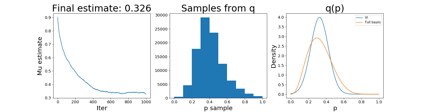
We can see that it finds a similar solution as the fully Bayesian approach, although we fixed the variance, which limits the flexibility of the variational approach.

MCMC

A second major family of approximations to full Bayesian inference is the class of Markov Chain Monte Carlo methods. The main idea behind this suite of methods is that we find ways to sample from the unnormalized posterior, and the collection of these samples then represent a finite approximation to the true posterior. Although this is still an approximation, in the limit of infinite samples (and some regularity conditions), we should be able to recover the true posterior. This stands in contrast to variational inference, where we will always be limited in how closely we can approximate the posterior depending on which variational family $Q$ we choose.

Most variants of MCMC differ in the way that they perform the sampling step. Here, let’s take a look at one of the most well-known MCMC algorithms, Metropolis-Hastings.

In Metropolis-Hastings, we iteratively sample from the support of the parameter of interest, with the intent that we explore regions of high density more. Then, the goal is that the resulting set of samples is representative of the true posterior distribution.

In particular, we start at a random point $\rho_0$ in the support, and then we sample new points around this point using a proposal distribution $g(\rho)$. We center the distribution $g(\rho)$ around $\rho_0$, then sample a new point $\hat{\rho}$. To decide whether to jump to $\hat{\rho}$ next, we check whether $\hat{\rho}$ is more probable under our model. Specifically, we compute the ratio

Notice that this lets us avoid computing the denominator directly.

An example for the Beta-Bernoulli model in Python is below, which uses a Gaussian proposal function.

## MCMC 

def beta_bernoulli_unnorm_posterior(x, p, a, b):
    return ((a - 1 + np.sum(X)) * np.log(p) + (b - 1 + np.sum(1 - X)) * np.log(1 - p))

curr_p = 0.1
n_iter = 1000
proposal_width = 0.1
burnin_len = 20

p_history = []
for ii in range(n_iter):
    
    # Unnormalized Beta-bernoulli log-posterior
    curr_lik = beta_bernoulli_unnorm_posterior(X, curr_p, a, b)
    
    # Propose new value of p using gaussian
    proposed_p = norm(curr_p, proposal_width).rvs()
    proposed_p = min(proposed_p, 1-1e-4)
    proposed_p = max(proposed_p, 1e-4)
    proposed_lik = beta_bernoulli_unnorm_posterior(X, proposed_p, a, b)
    
    # Check if we should accept this new value
    p_accept = proposed_lik - curr_lik
    accept = np.log(np.random.rand()) < p_accept
    
    if accept:
        curr_p = proposed_p
    
    # Only save values after some burn-in length
    if ii > burnin_len:
        p_history.append(curr_p)
        
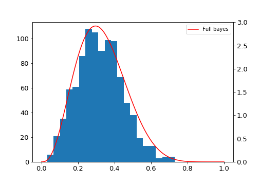
# p_history should now contain samples from the posterior

And the result:

Laplace approximation

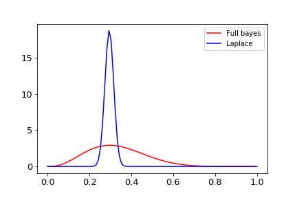
Finally, the Laplace approximation is a straightforward way to approximate the posterior: simply fit a Gaussian around the MAP estimate. In particular it can be shown by Taylor expansion that the distribution will be approximated by a Gaussian at its maximum.

In particular, we take the Gaussian’s mean to be the MAP estimate, and its variance to be the negative inverse of the second derivative at the MAP estimate (this essentially estimates the curvature at the maximum of the posterior.

An example for our Beta-Bernoulli example is shown in Python below:

## Laplace approximation

laplace_mean = map_estimate
second_deriv_ll = -1 / map_estimate**2 * (np.sum(X) + a - 1) - 1 / (1 - map_estimate)**2 * (np.sum(1 - X) + b - 1)
laplace_var = -1 / second_deriv_ll

And the result:

References

• Ranganath, Rajesh, Sean Gerrish, and David M. Blei. “Black Box Variational Inference.” Proceedings of the Seventeenth International Conference on Artificial Intelligence and Statistics. 2014.
• Prof. Surya Tapas Tokdar’s notes on the Laplace approximation