Andy Jones
Power posteriors
\(\DeclareMathOperator*{\argmin}{arg\,min}\) \(\DeclareMathOperator*{\argmax}{arg\,max}\)
Bayesian inference relies on transparent modeling assumptions to make conclusions about a dataset. Those assumptions are often (or always) wrong, which can affect the downstream conclusions we make. To combat this issue, many approaches have been proposed to make Bayesian inference “robust” to false assumptions. In this post, we explore one of these solutions: power posteriors.
Modeling setup
Suppose we observe a dataset $x = (x_1, \cdots, x_n)$ and we posit the following generic model with parameter(s) $\theta$:
\begin{align} x_i | \theta &\stackrel{ind}{\sim} p(x | \theta) \\ \theta &\sim \pi(\theta), \end{align}
where the first line describes the likelihood, and $\pi$ is a prior for $\theta$. A straightforward application of Bayes rule gives us the posterior for $\theta$:
\begin{equation}\label{eq:posterior} p(\theta | x) = \frac1Z p(x | \theta) \pi(\theta) = \frac1Z \pi(\theta) \prod\limits_{i=1}^n p(x_i | \theta), \tag{1} \end{equation}
where $Z = p(x) = \int_\Theta p(x | \theta) \pi(\theta) d\theta$ is a normalizing constant.
Power posteriors: The basic idea
The basic idea behind power posteriors is very simple: we raise the likelihood to a power $\gamma \in (0, 1).$ During inference, the posterior in Equation \eqref{eq:posterior} is then
\begin{equation}\label{eq:power_posterior} p(\theta | \mathbf{x}) = \frac1Z \pi(\theta) \prod\limits_{i=1}^n p(x_i | \theta)^\gamma. \tag{2} \end{equation}
Although it may not be clear why this is a good idea, it has a downstream effect of “robustifying” the statistical model to misspecification. We’ll explore this in a bit more depth below. Specifically, there are several ways to interpret this approach; here, we describe three interpretations, as laid out by Jeff Miller in a 2017 talk.
Synthetically reducing the sample size
In our modeling setup, we observed $n$ data samples. In the standard posterior (Equation \eqref{eq:posterior}), each sample contributed to the posterior through its likelihood $p(x_i | \theta)$. Vacuously, the likelihood of each sample was raised to the power of one in this standard posterior.
The power posterior in Equation \eqref{eq:power_posterior} effectively reducing the contribution of each sample to the posterior by raising the likelihoods to a power $\gamma$ that is between zero and one. We can view this as reducing the sample size from $n$ to $n \gamma.$
As a demonstration of this idea, consider the following simple two-layer Gaussian hierarchical model:
\begin{align} x_1, \dots, x_n &\sim \mathcal{N}(\mu, 1) \\ \mu &\sim \mathcal{N}(0, 1), \end{align}
and suppose we’re interested in estimating the mean $\mu$. Under standard Bayesian inference, the posterior is given by
\[\mu | x \sim \mathcal{N}\left(\frac{1}{n+1} \sum_i x_i, \frac{1}{n + 1} \right).\]On the other hand, if we were to use the power posterior, we would have
\[\mu | x \sim \mathcal{N}\left(\frac{\gamma}{n+1} \sum_i x_i, \frac{1}{\gamma n + 1} \right).\]Let’s now visualize the difference between these two posteriors. Suppose the true mean is $\mu^\star = 1.5,$ and we observe $n=10$ data points from the model. In the plot below, we show the data as gray ticks at the bottom, the standard posterior in black, and the power posterior in red. We set $\gamma=0.5$ in this experiment.
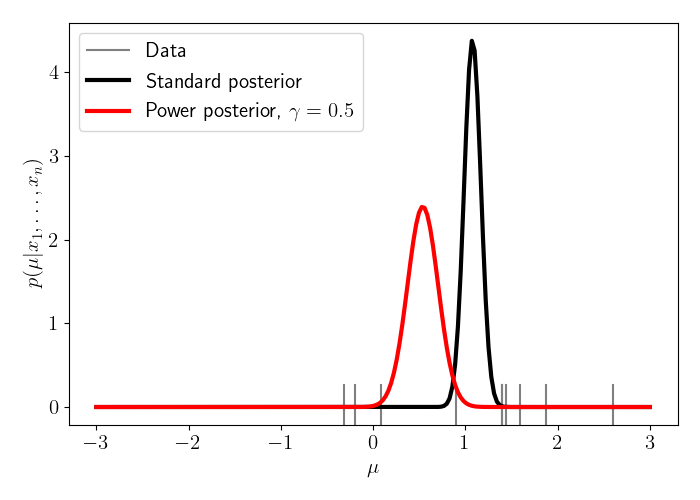
We can notice how the power posterior “regularizes” the standard posterior, in the sense that it downweights the likelihood, which effectively upweights the contribution of the prior. In this case, we see that the power posterior is shifted toward zero and has a higher variance compared to the standard posterior. Of course, in this case it’s worth noting that our model isn’t misspecified (in fact, it’s perfectly specified), so applying the power posterior in this setting is misguided. Nevertheless, this simple example helps build intuition.
We can also imagine that we observe the $n=10$ data points sequentially and observe how each of these posteriors updates with each sample. The animation below shows exactly this, where each data point is observed in sequence.
We can see that the power posterior updates more “slowly” in a sense, whereas the standard posterior concentrates its mass fairly quickly.
Penalizing model complexity
A second way to interpret the power posterior is to more explicitly cast it as a form of regularization. In particular, we can view the power posterior as an objective that balances the goodness of fit to the data and the overall complexity of the model.
To see this, consider that one way to perform inference is to attempt to maximize the marginal likelihood of the data. The marginal likelihood is the likelihood of the data, where the model parameters have been integrated out. If we denote our model as $\mathcal{M}$, then in our notation, the marginal likelihood is given by
\[p(x | \mathcal{M}) = \int_{\Theta} p(x | \theta, \mathcal{M}) \pi(\theta | \mathcal{M}) d\theta.\]This quantity also appears as the normalizing constant in the standard posterior (Equation \eqref{eq:posterior}).
In an ideal world, we could maximize this quantity over models $\mathcal{M}.$ If our space of models is given by $\mathscr{M}$, then this optimization problem would be:
\[\mathcal{M}^\star = \argmax_{\mathcal{M} \in \mathscr{M}} p(x | \mathcal{M}).\]In practice, this is an intractable problem for multiple reasons. The most pressing problems are that the integral above is typically intractable, and that deciding on a reasonable space of models $\mathscr{M}$ is difficult. Nevertheless, we can analyze this quantity to build intuition about the differences between the standard posterior and the power posterior.
To do this, let’s make a simple approximation of the marginal likelihood. This simple trick largely follows the one used in Section 3.4 of Bishop’s PRML textbook. To start, assume that the posterior is peaked around its maximum value $\theta_{\text{MAP}}$, and that this peak has width $\Delta \theta_{\text{posterior}}$. Moreover, assume that the prior $\pi$ is effectively flat over a wide region of width $\Delta \theta_{\text{prior}}$, so we have $p(\theta) \approx \frac{1}{\Delta \theta_{\text{prior}}}$. Then, we can approximate the integral in the marignal likelihood using simple area estimates. In particular, omitting the references to $\mathcal{M}$ for clarity, we have
\[p(x) = \int_{\Theta} p(x | \theta) \pi(\theta) d\theta \simeq p(x | \theta_{\text{MAP}}) \frac{\Delta \theta_{\text{MAP}}}{\Delta \theta_{\text{prior}}}.\]Taking a log, we have
\[\log p(x) \simeq \underbrace{\log p(x | \theta_{\text{MAP}})}_{\text{Fit to data}} + \underbrace{\log \left(\frac{\Delta \theta_{\text{MAP}}}{\Delta \theta_{\text{prior}}}\right)}_{\text{Complexity penalty}}.\]The first term here measures the model’s goodness of fit to the data, and the second term penalizes complex models. Since $\Delta \theta_{\text{MAP}} < \Delta \theta_{\text{prior}}$, the complexity term will always be negative. Notice that if the model fits the data extremely well, the posterior will be sharply peaked, and $\Delta \theta_{\text{MAP}}$ will be small, resulting in a large penalty.
Making this same approximation in the power posterior setting, we have
\[\log p(x) \simeq \color{red}{\gamma} \log p(x | \theta_{\text{MAP}}) + \log \left(\frac{\Delta \theta_{\text{MAP}}}{\Delta \theta_{\text{prior}}}\right).\]This marginal likelihood is identical to the one for the standard posterior, except we have an extra weighting term $\gamma$ on the goodness of fit term. Since $\gamma$ is between zero and one, this has the effect of increasing the relative contribution of the penalty term on the right.
We can visualize this below, similar to Figure 3.12 in Bishop’s textbook.
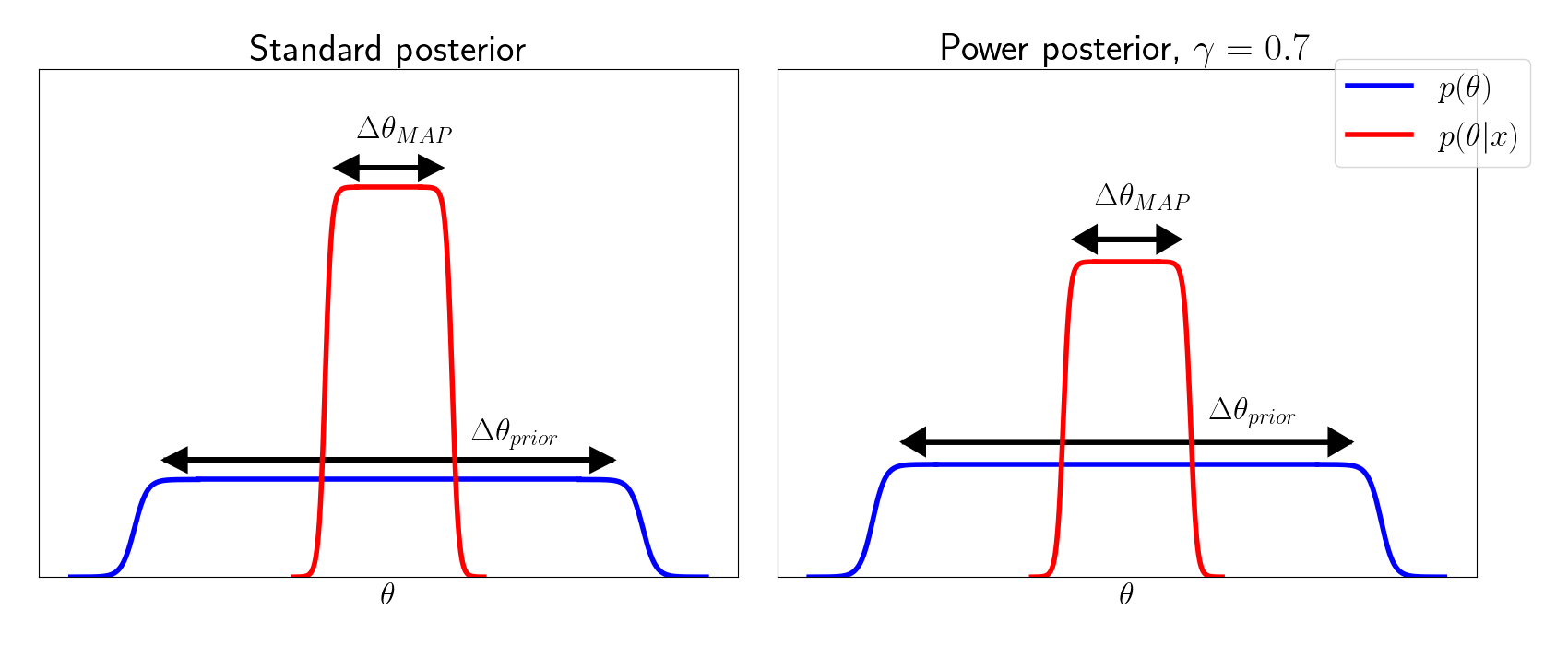
We see that, while the prior doesn’t change between the two posteriors, the power posterior reduces the likelihood of the data under the MAP value.
Approximation to the coarsened posterior
Coarsened posteriors were introduced by Miller and Dunson as a way to account for model misspecification in a principle Bayesian fashion. Whereas a standard Bayesian posterior conditions on a set of observed data points, the coarsened posterior conditions on the event that the observed data did not come from the model being posited.
More specifically, let’s denote our $n$ observed data distribution as $\hat{P}_{x_{1:n}} = \sum_{i=1}^n \delta_{x_i}$ and the “idealized data distribution” (the data distribution that would be observed if the model were correct) as $\hat{P}_{X_{1:n}}$. Then, the c-posterior conditions on the event that these two distributions are in a neighborhood of width $r$ of each other:
\[p(\theta | d(\hat{P}_{X_{1:n}}, \hat{P}_{x_{1:n}}) < R)\]where $d$ is a divergence measure.
Now suppose that the data distribution is given by $p_o$ and the idealized distribution is given by $p_\theta$. We can place an exponential prior on $R \sim \text{Exp}(\alpha)$, the coarsened posterior is then proportional to
\[p(\theta | d(p_o, p_\theta) < R) \propto p(d(p_o, p_\theta) < R | \theta) \cdot \pi(\theta).\]We can notice that $p(d(p_o, p_\theta) < R | \theta)$ is essentially one minus the CDF of $R$, and since $R$ has an exponential prior, we can write this as
\[p(d(p_o, p_\theta) < R | \theta) = \exp(-\alpha d(p_o, p_\theta)).\]If we take $d$ to be the KL divergence, we then have
\[\exp(-\alpha \int p_o \log p_\theta).\]We can then put the prior back in and approximate the integral with a sum over our finite dataset. In the process, the $p_o$ term is absorbed by the normalizing constant, and we have the following approximation:
\begin{align} \exp\left\{ -\alpha d(p_o, p_\theta) \right\} \pi(\theta) &\propto \exp\left\{ \alpha \int p_o \log p_\theta \right\} \pi(\theta) \\ &\approx \exp\left\{ \frac{\alpha}{n} \sum\limits_{i=1}^n \log p_\theta (x_i) \right\} \pi(\theta) & \text{Approximate with sum} \\ &= \pi(\theta) \prod\limits_{i=1}^n p_\theta(x_i)^{\alpha / n}. \end{align}
We can see that the last term is exactly the power posterior, with $\gamma = \alpha/n$. Thus, the coarsened posterior is a generalization of the power posterior, where the power posterior corresponds to a special approximation to the case when $R \sim \text{Exp}(\alpha)$ and the divergence measure is the KL divergence.
Code
The code for producing the visualizations in this post can be found in this GitHub repo.
References
- Miller, Jeffrey W., and David B. Dunson. “Robust Bayesian inference via coarsening.” Journal of the American Statistical Association (2018).
- Jeff Miller’s 2017 talk at BNP.
- Bishop, Christopher M. “Pattern recognition.” Machine learning 128.9 (2006).