Andy Jones
Power iteration method
The power iteration algorithm is a numerical approach to computing the top eigenvector and eigenvalue of a matrix.
Background
Consider a diagonalizable matrix $A \in \mathbb{R}^{n \times n}$ with eigenvalue decomposition
\[A = V \Lambda V^{-1}.\]In this notation, the columns of $V$ contains the eigenvectors of $A$, and $\Lambda = \text{diag}(\lambda_1, \dots, \lambda_n)$ contains the corresponding eigenvalues with $|\lambda_1| > \cdots > |\lambda_n|$.
Consider what happens when we take powers of $A$:
\begin{align} A &= V \Lambda V^{-1} V \\ AA = V \Lambda V^{-1} V \Lambda V^{-1} &= V \Lambda^2 V^{-1} \\ AAA = V \Lambda V^{-1} V \Lambda V^{-1} V \Lambda V^{-1} &= V \Lambda^3 V^{-1} \\ &\vdots \\ \underbrace{A \cdots A}_{\text{$k$ times}} &= V \Lambda^k V^{-1}. \\ \end{align}
In the above, powers of $\Lambda$ are equivalent to $\Lambda^k = \text{diag}(\lambda_1^k, \dots, \lambda_n^k)$.
Method
Consider a random vector $\mathbf{b} \in \mathbb{R}^n$. Note that $\mathbf{b}$ can always be written as a linear combination of $A$’s eigenvectors:
\[b = \sum\limits_{i=1}^n \mathbf{v}_i b_i = V\widetilde{\mathbf{b}}\]where $\widetilde{\mathbf{b}} = (\widetilde{b}_1, \dots, \widetilde{b}_n)^\top$ is another vector.
Now, let’s rewrite $A^k \mathbf{b} = A^k V \widetilde{\mathbf{b}}$ as a sum over eigenvalues and eigenvectors:
\[A^k V \widetilde{\mathbf{b}} = V \Lambda^k V^{-1} V \widetilde{\mathbf{b}} = V \Lambda^k \widetilde{\mathbf{b}} = \sum\limits_{i=1}^n \mathbf{v}_i \lambda_i^k \widetilde{b}_i.\]Now, to understand how the top eigenvalue relates to the others, let’s pull out $\lambda_1$:
\begin{equation} \label{eq:eq1} A^k V \widetilde{\mathbf{b}} = \lambda_1^k \sum\limits_{i=1}^n \mathbf{v}_i \left(\frac{\lambda_i}{\lambda_1}\right)^k \widetilde{b}_i. \end{equation}
With each power of $A$, the value of $\left(\frac{\lambda_i}{\lambda_1}\right)^k$ will decrease, eventually going to zero as $k \to \infty$. In other words, as $k\to \infty$,
\[A^k V \widetilde{\mathbf{b}} \to \mathbf{v}_1 \lambda_1^k b_1.\]This means that $A^k V \widetilde{\mathbf{b}} = A^k \mathbf{b}$ will converge to a vector that is a scalar multiple of the top eigenvector (multiplied by $\lambda_1^k b_1$). Thus, all that’s left to do is normalize this expression to make it a unit vector, and we’re left with
\[\frac{A^k \mathbf{b}}{\|A^k \mathbf{b}\|_2}.\]Putting it all together, we have the full power method:
- Draw random $n$-vector $\mathbf{b}_0$.
- Set $\mathbf{b}_1 := A \mathbf{b}_0$.
- For $k=2, \dots, K$: 3.1. Set $\widehat{\mathbf{b}}_k := A \mathbf{b}_{k-1}$. 3.2 Normalize by setting $\mathbf{b}_k = \frac{\widehat{\mathbf{b}}_k}{||\widehat{\mathbf{b}}_k||_2}$.
- Return $\mathbf{b}_K$.
Experiments
The power iteration method can be implemented fairly easily in Python. Below is some sample code for finding the top eigenvector for a given matrix A.
num_iters = 100

# Starting vector
b = np.random.rand(A.shape[0])

# Power iteration
for ii in range(num_iters):

    # Project
    bnew = A @ b

    # Normalize
    b = bnew / np.linalg.norm(bnew, ord=2)
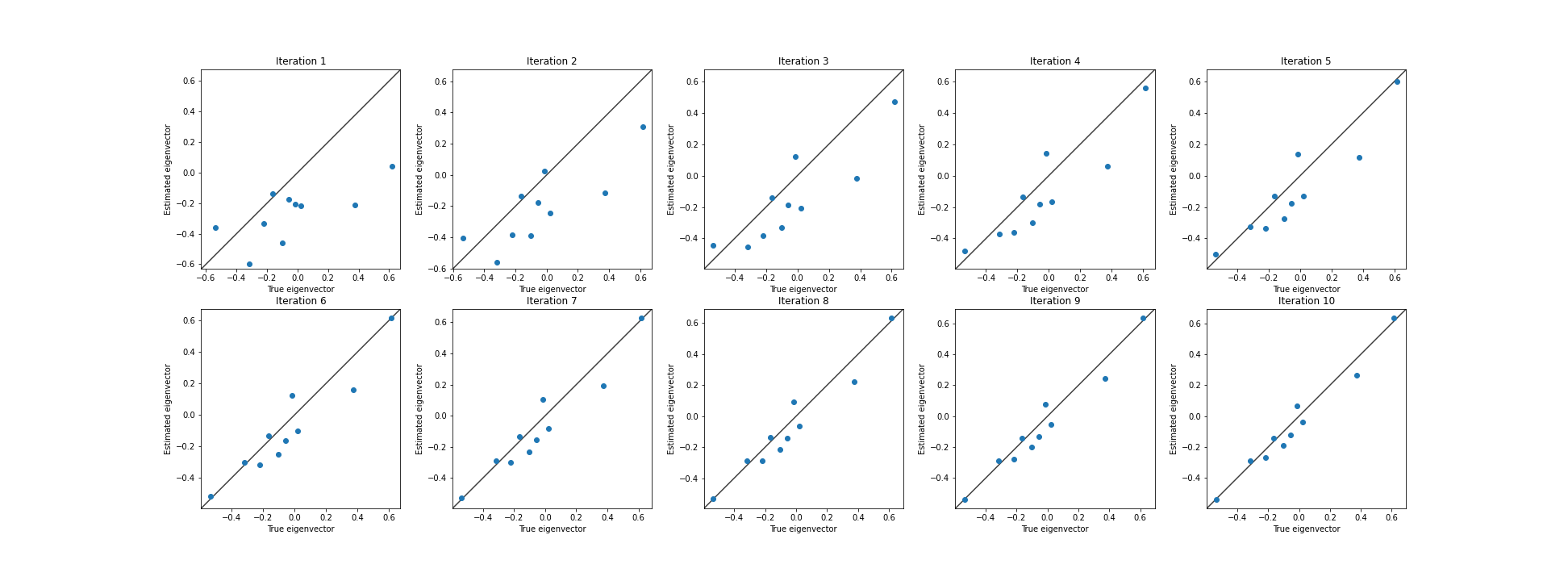
Testing this on a random $10 \times 10$ matrix, we can see that the estimated top eigenvector quickly approaches the true top eigenvector. Below, we plot each element of the eigenvector as a point.
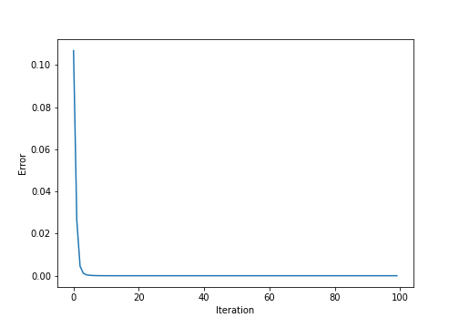
We can view this convergence another way by estimating the mean-squared error (MSE) at each iteration.
However, it’s important to note that the rate of convergence of this method will depend on a few factors. One of the most important is how tightly “spiked” the top eigenvalue is. In particular, if $|\lambda_1| \gg |\lambda_2|$, then it will quickly converge. However, if these are close to one another, it will take longer. Intuitively, this is because the ratio $\frac{\lambda_2}{\lambda_1}$ in \eqref{eq:eq1} will take longer to go to zero.
We can show this phenomenon numerically by fixing the eigenvectors of a matrix and varying the difference between $\lambda_1$ and $\lambda_2$. Below, we plot the error over iterations, with each line representing a different set of eigenvalues. The legend shows the value $|\lambda_1| - |\lambda_2|$.
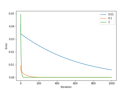
Clearly, as the top eigenvalue becomes more dominant, the power iteration method converges faster.
References
- Prof. David Bindel’s notes on the power iteration method.
- Wikipedia page on the power iteration method.