Andy Jones
Posterior consistency
Bayesian models provide a principled way to make inferences about underlying parameters. But under what conditions do those inferences converge to the truth?
Frequentist consistency
The consistency of estimators is usually discussed in the context of classical frequentist statistics. In that regime, a consistent estimator is one that converges in probablility to the true parameter as the number of data points approaches infinity. More precisely, an estimator $\widehat{\theta}_n$ is consistent if
\[\widehat{\theta}_n \to_p \theta_0,\]where $\theta_0$ is the true parameter value.
Posterior consistency
The idea of consistency can also be extended to the Bayesian world. Here, we consider inferences for $\theta$ made under the posterior distribution for some model, $p(\theta | X)$. Since the estimator is no longer a point estimate, but rather a distribution, we need a new definition of “consistency” in this setting.
Roughly, a posterior is considered consistent if it eventually concentrates as a point mass around the true value $\theta_0$. Furthermore, for consistent estimators, we’re often interested in “how fast” this happens (or the so-called “rate of convergence”).
Consider the following generic Bayesian model for data $x_1, \dots, x_n$ with parameter (or parameter vector) $\theta \in \Theta$:
\begin{align} x_i &\sim p(x | \theta) \\ \theta &\sim \pi(\theta). \end{align}
Let’s say the true parameter that generated the data is $\theta_0 \in \Theta$.
When we observe $n > 0$ data points $X_n = {x_1, \dots, x_n}$, we can compute the posterior, denoted $\Pi_n$ here:
\[\Pi_n := p(\theta | X_n) = \frac{p(X_n | \theta) p(\theta)}{\int_\Theta p(X_n | \theta) p(\theta) d\theta}.\]It’s now reasonable to ask how “close” $\Pi_n$ gets to the true parameter value $\theta_0$, especially as $n \to \infty$.
Similar to the frequentist setting, we typically talk about a “sequence” of posteriors ${\Pi_n}$, each one corresponding to a particular value of $n$. As $n$ increases, we see more data, and ideally the posterior converges to the truth, which is a point mass $\delta_{\theta_0}$.
For example, consider the following simple Gaussian model with unknown mean $\mu$ and known variance $\sigma^2=1$:
\begin{align} x_i \sim \mathcal{N}(\mu, 1) \\ \mu \sim \mathcal{N}(0, 1). \end{align}
The posterior for $\mu$, $p(\mu | X)$ has a closed form, and we can consider how this posterior changes for $n=1, 2, \dots$. Below, I plotted the posterior for increasing values of $n$, with darker colors representing higher values of $n$. Here, I generated the data with $\mu=1$.
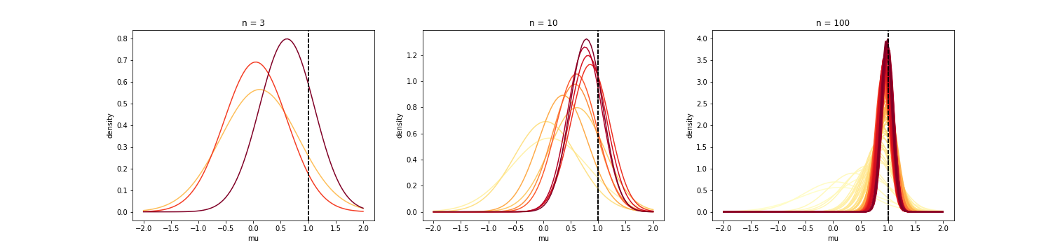
We can see that, as $n$ increases, the posterior starts to concentrate around the true value of $\mu$, which is $1$ in this case. Posterior consistency is a concept that formalizes this idea of concentrating around the true value. Below, we define and discuss posterior consistency two ways: in terms of distance, and in terms of neighborhoods.
Consistency in terms of distance
Roughly, the first characterization of consistency says that the posterior should get closer and closer the the true parameter value as we see more data. To more precisely defined closeness, we need to define a metric $d$ that measures the distance between distributions. A common one is the Wasserstein distance. Then, we can define consistency more formally as follows.
${\Pi_n}$ is consistent for $\theta_0$ if $d(\Pi_n, \delta_{\theta_0}) \to 0 \text{ almost surely.}$
Here, $\delta_{\theta_0}$ is a point mass at $\theta_0$. Intuitively, this definition says that a consistent posterior should become indistinguishable from a point mass at the true parameter as $n$ increases.
Consistency in terms of neighborhoods
Another useful and equivalent way to define posterior consistency is in terms of “neighborhoods” around $\delta_{\theta_0}$. Specifically, we define a “weak” $\epsilon$-neighborhood $U_\epsilon(\theta_0)$ around $\theta_0$ as
\[U_{\epsilon, w}(\theta_0) = \{\theta \in \Theta : |\smallint f(\theta) - \smallint f(\theta_0)| < \epsilon\}.\]Similarly, a “strong” $\epsilon$-neighborhood around $\theta_0$ is
\[U_{\epsilon, s}(\theta_0) = \{\theta \in \Theta : \|\theta - \theta_0\|_1 < \epsilon\}.\]Using neighborhoods, we have a second characterization of consistency:
$\Pi_n$ is consistent if and only if for every open neighborhood $U$ of $\theta_0$, $\Pi_n(U^c | X_n) \to 0 \text{ almost surely.}$
Intuitively, this means that a consistent posterior places no mass outside of the truth. In the definition above, $\Pi_n$ can either obey strong or weak consistency depending on the type of neighborhood.
Schwartz’s theorem
In 1965, Lorraine Schwartz proved a very general theorem giving sufficient conditions under which a posterior is consistent.
To do this, he used the idea of “test functions”, which are closely tied to decision theory. In this setting, a test function $\Phi_n(X_n)$ is a function of the data that maps to $[0, 1]$.
Now, consider two types of worlds: one in which the data was generated by $\theta_0$, and many others in which the data wasn’t generated by $\theta_0$. Intuitively, if a posterior is consistent, we should be able to construct test functions that can discriminate between these two scenarios as $n \to \infty$. In particular, if $\theta_0$ is the true parameter, we should be able to classify or decide whether some data $X_n$ was generated from $\theta_0$ or not.
We can view this in terms of a hypothesis testing framework as well. Consider the following null and alternative hypotheses:
\[H_0: \theta = \theta_0, ~~~~~ H_1: \theta \neq \theta_0.\]Then we want to be able to construct a decision rule such that the two types of error are low: $\mathbb{P}[\text{reject }H_0 | H_0 \text{ is true}]$ and $\mathbb{P}[\text{accept }H_0 | H_1 \text{ is true}]$.
Since the output of our test functions $\Phi_n$ is in $[0, 1]$, let’s think about its output as the probability that we reject $H_0$ (i.e., $\Phi_n$ gives us a randomized decision rule). Then clearly we want $\Phi_n(X_n)$ to be low when $\theta = \theta_0$ and high when $\theta \neq \theta_0$. We write this in terms of expectations:
- Want to be close to $0$: $\mathbb{E}_{\theta_0}[\Phi_n(X_n)]$
- Want to be close to $1$: $\mathbb{E}_{\theta_0^c}[\Phi_n(X_n)]$ (equivalently, want $\mathbb{E}_{\theta_0^c}[1 - \Phi_n(X_n)]$ to be close to $0$)
At this point, we almost have all the ingredients for Schwartz’s theorem. The last concept to define is KL support. We say that $\theta_0$ belongs to the KL support of a prior $\pi$ if for every $\epsilon > 0, \pi({ \theta : d_{KL}(\theta_0, \theta) < \epsilon }) > 0$. Roughly, $\theta_0$ is in the KL support of $\pi$ if there’s any prior mass at $\theta_0$ (a fairly loose condition, which is nice).
At this point, we’re ready to state Schwartz’s theorem:
Theorem. If $\theta_0$ belongs to the KL support of $\pi$, and $U_n \subset \mathcal{F}$ are neighborhoods of $\theta_0$ such that there are test functions $\Phi_n, n=1,2,\dots$ satisfying
\[\mathbb{E}_{\theta_0}[\Phi_n(X_n)] \leq Be^{-bn} \text{ and } \sup_{\theta \in U_n^c} \mathbb{E}_\theta[1 - \Phi_n(X_n)] \leq B e^{-bn}\]for some constants $b, B > 0$, then $\Pi_n$ is consistent.
Intuitively, this result says that if $\theta_0$ is in the support of the prior, and we can classify $\theta_0$ vs. $\theta_0^c$ as we get more data, then the posterior is consistent. The particular bound of $Be^{-bn}$ is typically known as “exponential consistency” for the test $\Phi_n$.
In the theorem, we can think of the first condition as the probability of incorrectly rejecting the null hypothesis (deciding $\theta = \theta_0$ when $\theta \neq \theta_0$), and the second condition as the probability of incorrectly accepting the null hypothesis (deciding $\theta \neq \theta_0$ when $\theta = \theta_0$).
Code
Below is the code for generating the plot of posterior distributions for the Gaussian model in the first section above.
import numpy as np
import matplotlib.pyplot as plt
from scipy.stats import norm

def get_gaussian_mean_posterior(X, sigma2, mu_0, sigma2_0):
    n = X.shape[0]

    # Compute MLE
    mu_mle = np.mean(X)

    # Get posterior mean as weighted combination of prior and MLE
    prior_weight = sigma2 / (n * sigma2_0 + sigma2)
    mle_weight = n * sigma2_0 / (n * sigma2_0 + sigma2)
    posterior_mean = prior_weight * mu_0 + mle_weight * mu_mle

    # Get posterior variance
    posterior_precision = 1 / sigma2_0 + n / sigma2
    posterior_var = 1 / posterior_precision

    return posterior_mean, posterior_var

def plot_gaussian_pdf(ax, mean, var, xlims=[-2, 2], label="", color="black"):
    xs = np.linspace(xlims[0], xlims[1], 100)
    pdf_vals = norm.pdf(xs, loc=mean, scale=np.sqrt(var))
    ax.plot(xs, pdf_vals, label=label, color=color)

# Set up true parameters
n_list = [3, 10, 100]
sigma2 = 1
mu_true = 1
mu_0 = 0
sigma2_0 = 1

# Generate data one-by-one and plot posterior with each incoming sample
X = np.random.normal(mu_true, sigma2, size=n)
plt.figure(figsize=(21, 5))
colormap = plt.get_cmap("YlOrRd")

for jj, n in enumerate(n_list):
    plt.subplot(1, len(n_list), jj + 1)
    ax = plt.gca()
    for ii in range(n):
        x = X[:ii+1]
        posterior_mean, posterior_var = get_gaussian_mean_posterior(x, sigma2, mu_0, sigma2_0)
        plot_gaussian_pdf(ax, posterior_mean, posterior_var, label="n={}".format(ii+1), color=colormap(int(255./n * (ii + 1))))

        plt.axvline(mu_true, color="black", linestyle="--")
    plt.xlabel("mu")
    plt.ylabel("density")
    plt.title("n = {}".format(n))
plt.show()