Monge and Kontorovich formulations of the Optimal Transport problem

\(\DeclareMathOperator*{\argmin}{arg\,min}\) \(\DeclareMathOperator*{\argmax}{arg\,max}\)

Transportation theory studies the mathematical and algorithmic analysis of the physical movement of goods and resource allocation. The field of optimal transport is concerned with finding routes for these movements that minimize some type of cost.

Preliminaries

We denote a discrete density over a support at $n$ different locations $x_1, \dots, x_n$ as

where $\delta_{x_i}$ is a Dirac point mass at location $x_i$ and $\mathbf{a} = (a_1, \cdots, a_n)^\top$ is a vector of weights for each position. We constrain the weights to sum to one, $\sum_{i=1}^n a_i = 1$, and thus $\mathbf{a}$ lies on a $n$-dimensional simplex, which we denote as $\mathbf{a} \in \Delta^n$.

Optimal transport

At a general level, the optimal transport (OT) problem is to transform one density into another density while minimizing the transportation cost. There are two major formulations of OT — one developed by Gaspard Monge and the other by Leonid Kontorovich. We explore both of these viewpoints below.

Monge formulation

The Monge formulation of optimal transport restricts itself to transportation between two uniform discrete densities whose support has the same size $n$. In particular, it seeks a mapping from one density $\alpha$ to another $\beta$, where

and $a_1 = \cdots = a_n = b_1 = \cdots b_n = \frac1n$. Note that the supports of the two densities, $\{x_i\}_{i=1}^n$ and $\{y_j\}_{j=1}^n$, may not be the same, and in fact need not be overlapping at all.

Furthermore, we assume that there is a cost associated with assigning a mass at $x_i$ to be transported to $y_i$. In this case, we can represent this cost function as a matrix $\mathbf{C} \in \mathbb{R}_+^{n \times n}$. The $ij$’th element, $\mathbf{C}_{ij}$ will be a nonnegative scalar representing the cost of transporting from $x_i$ to $y_j$.

In this simple case, the optimal transport problem reduces to a problem of “matching,” where we’d like to pair each $x_i$ with a single $y_j$ such that the cost is minimized. Formally, we can identify this as a problem of finding a permutation $\sigma : [n] \rightarrow [n]$ that maps the indices $1, \dots, n$ to the indices $1, \dots, n$.

Taking the set of valid permutations to be $\text{Perm}(n)$, one way to write the optimization problem is:

Kontorovich formulation

The Kontorovich version of optimal transport is a strict generalization of the Monge version. Rather than assuming that each mass is transported to just one other location, the Kontorovich problem allows for it to be split among multiple locations. Furthermore, it no longer requires each density to be uniform over the same size support.

To formalize this problem, consider again two discrete densities,

where $n \neq m$ in general, and $\mathbf{a}$ and $\mathbf{b}$ are any two $n$- and $m$-dimensional (respectively) positive vectors.

The goal is now to find a matrix $\mathbf{P} \in \mathbb{R}_+^{n \times m}$ whose $ij$’th element is a scalar representing the amount of mass at location $x_i$ that shuold be transported to location $y_j$.

Importantly, we have extra constraints on this matrix: We must ensure that mass is conserved in the transportation plan. In other words, the total amount of mass distributed from $x_i$ to all target locations must equal $a_i$, and the amount of mass distributed to $y_j$ from all source locations must be equal to $b_j$. Stating this mathematically, we can write the set of admissible transport plans as

Extension to continuous distributions

All of the above descriptions have focused on discrete densities. However, we can also consider the problem of transporting one continuous density to another continuous density. (Semi-discrete OT problems also exist, where a continuous density is transported to a discrete density.)

This case is described most easily in terms of marginal and joint distributions. We observe two marginal distributions $p(x)$ and $p(y)$, and we’re interested in finding a transport plan that maps $p(x)$ to $p(y)$. In the continuous case, this plan can be described with a joint density over both $x$ and $y$. The set of admissible joint densities is given by:

Notice that this constraint is simply a generalization of the mass preservation constraint in the discrete case. Here, mass conservation is framed in terms of a joint distribution having particular marginal densities.

Examples

Discrete densities

To start with a simple example, consider the two discrete densities in the plot below, where $p(x)$ is made up of two point masses, and $p(y)$ is made up of three point masses.

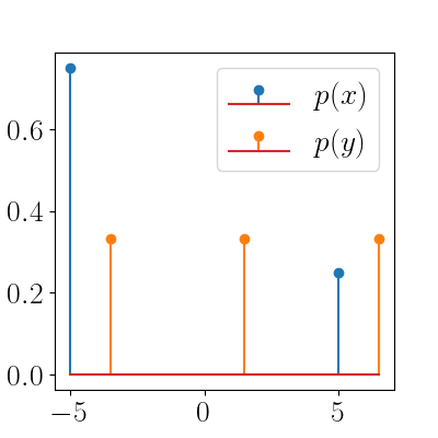
Again, the goal of an optimal transport problem in this case is to transfer the blue masses to the orange masses in the most “efficient” way possible. Here, we can solve this with a simple linear program. Suppose our cost function is the squared Euclidean distance, $c(x, y) = |x - y|^2$. In other words, the cost of transporting a mass from location $x$ to $y$ is the squared distance between them.

Suppose the domain of $x$ has support over $n$ locations and the domain of $y$ is over $m$ locations. Here, we can represent our cost function as a matrix $\mathbf{C} \in \mathbb{R}^{n \times m}$, where $\mathbf{C}_{ij} = c(x_i, y_j)$. Our optimation program is then

\begin{align} &\min_{\mathbf{T} \in \mathbb{R}^{n \times m}_+} \mathbf{T} \odot \mathbf{C} \\ \text{subject to }& \sum\limits_{i} \mathbf{C}_{ij} = p(y_j)~~ \forall j = 1,\dots, m \\ & \sum\limits_{j} \mathbf{C}_{ij} = p(x_i) ~~\forall i = 1,\dots, n. \end{align}

We have a linear objective and linear constraints, so we can solve this with out-of-the-box linear programming tools. Using SciPy’s tools, we can solve it with the code below. Because SciPy only supports matrix-vector equations of the form $\mathbf{A}\mathbf{x}=\mathbf{b}$, we flatten all matrix-matrix constraints to satisfy this form, then reshape at the end.

import numpy as np
from scipy.optimize import linprog
from sklearn.metrics import pairwise_distances

lims = [-5, 5]
nx = 2
ny = 3
p = 1

## Locations
x = np.linspace(lims[0], lims[1], nx)
y = np.linspace(lims[0], lims[1], ny) + 0.5

## Mass at each location
x_masses = [0.75, 0.25]
y_masses = [1./ny] * ny

## Cost function (matrix)
dists = pairwise_distances(x.reshape(-1, 1), y.reshape(-1, 1))
dists_flat = np.ndarray.flatten(dists)

## Set up the equality constraints
A = np.zeros((nx + ny - 1, nx * ny))
for nn in range(nx):
  A[nn, (nn*ny):((nn+1)*ny)] = 1
for nn in range(ny - 1):
  for nn2 in range(nx):
    A[nx + nn, nn2*ny + nn] = 1

b = np.concatenate([x_masses, y_masses[:-1]])

## Solve with interior point method
res = linprog(dists_flat, A_eq=A, b_eq=b)

## Reshape into matrix of transport plan
transport_plan = np.reshape(res.x, [nx, ny])

We can now check what the transport plan looks like. Below is a heatmap of the plan.

We can see that all of the mass of $p(x)$ at $x=5$ will be transferred to the rightmost location of the support of $y$ (which is closest in the Euclidean sense), and the mass of $p(x)$ of the left will spread itself out among the remaining masses of $p(y)$.

Consider another higher-dimensional, yet still simple, problem. Here, we have $10$ masses in each distribution, as shown in the stem plot below.

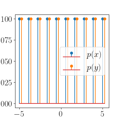
Each of the distributions is uniform, and we expect the optimal transport plan to be the one that simply shifts the nearby masses in $p(x)$ to the closes ones in $p(y)$. We can plot the transport map over time as the algorithm progresses (an interior point method provided by SciPy in this case). The animation below shows this.

We can see that the solver quickly reaches the optimum, which in this case transports mass only along the diagonal of the heatmap.

Continuous densities

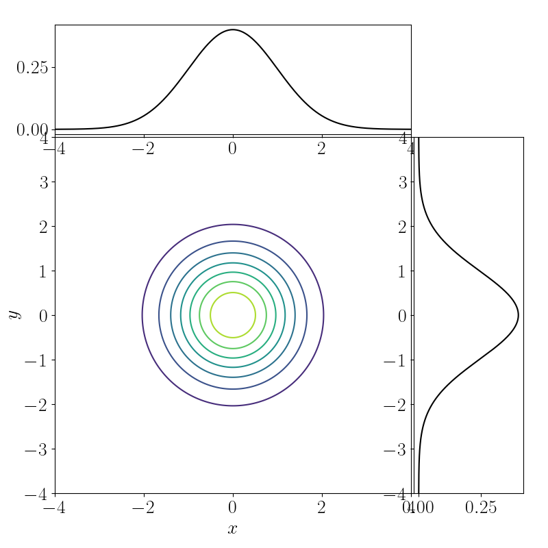
As shown above, OT also applies to the setting with continuous densities. As a simple example, consider two densities,

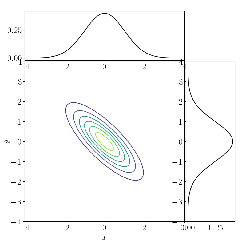
These marginals are plotted below, and we’d like to find the joint $p(x, y)$ that minimizes a cost.

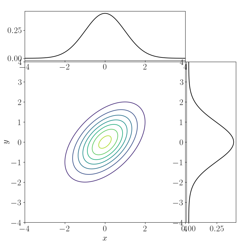
Note that there are infinitely many joint distributions that are consistent with having observed these marginals. Below we’ve plotted the contours three such two-dimensional densities.

Let the cost be the squared Euclidean distance:

Then our optimization problem is

\begin{align} \min_{p(x, y)} \int c(x, y) p(x, y) dx dy &= \min_{p(x, y)}\mathbb{E}_{p(x, y)}\left[ c(x, y) \right] \\ &= \min_{p(x, y)}\mathbb{E}_{p(x, y)}\left[ \|x - y\|^2 \right]. \end{align}

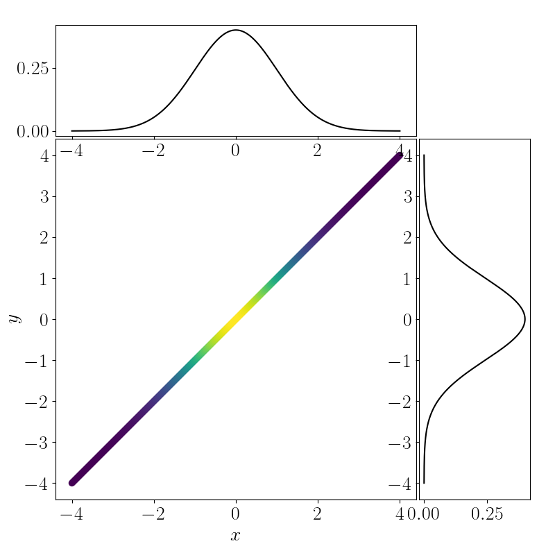
In this case, it becomes obvious that the optimal transport plan is to “do nothing.” In other words, to transport $p(x)$ to $p(y)$, we don’t have to do anything. More concretely, the optimal joint density will be a multivariate normal distribution with covariance

with $u, v \rightarrow 1$. This is effectively a one-dimensional Gaussian, as plotted below.

References

• Peyré, Gabriel, and Marco Cuturi. “Computational optimal transport: With applications to data science.” Foundations and Trends® in Machine Learning 11.5-6 (2019): 355-607.
• Matthew Thorpe’s Optimal Transport Notes