Nyström approximation

\(\DeclareMathOperator*{\argmin}{arg\,min}\) \(\DeclareMathOperator*{\argmax}{arg\,max}\)

Numerical linear algebra relies on performing fast and efficient calculations with matrices. However, when matrices become very large, computational bottlenecks can arise even for the most efficient numerical linear algebra techniques. Thus, there’s a need for methods that circumvent these bottlenecks by performing approximations that trade accuracy for computational efficiency.

In this post, we describe one of the simplest and most general approximations, widely known as the Nyström approximation. We focus on the case of positive definite covariance matrices, although similar approximations have been made in more general cases.

Covariance matrices

Suppose we have $n$ data points $x_1, \dots, x_n$. Let $K$ be an $n \times n$ covariance matrix (which we will also refer to as a kernel matrix), where $[K]_{ij} = k(x_i, x_j)$, and $k$ is a positive definite kernel function.

When $n$ is large, performing operations with $K$ will be expensive (recall that matrix storage costs $O(n^2)$ and matrix inversion costs $O(n^3)$). Thus, it’s of interest to find cheaper ways to approximate this kernel matrix, which can make downstream operations more efficient. The Nyström approximation is one such approach, which we explore next.

Nyström approximation

The basic idea behind the Nyström approximation is to describe the covariance matrix in terms of a smaller number of points. A full $n \times n$ covariance matrix describes the relationship between all $\frac{n^2 - n}{2}$ pairs of points, which can be expensive when $n$ is large. On the other hand, the Nyström approximation selects $m < n$ points (which we’ll call the “representative” points here) and approximates the covariance matrix by describing each of the original point’s relationship to these $m$ representative points.

More conceretly, a Nyström approximation makes the assumption that $\text{rank}(K) = m < n$. By making this low-rank assumption, we can avoid having to work with the full large $n \times n$ matrix.

External represenatative points

To see how this works in practice, suppose we randomly choose $m$ new points to be the “representative” samples of the dataset. Let’s call these points $\widetilde{x}_1, \dots, \widetilde{x}_m$. Then we can augment $K$ with these new points in the form of a block matrix:

where $K_{11}$ is the $m \times m$ kernel matrix for our representative points, $K_{22} = K$ is our $n \times n$ kernel matrix for the original points, and $K_{12}$ is the $m \times n$ kernel matrix for the cross-dataset covariances.

Let’s write $\widetilde{K}$ in terms of its SVD:

Using this decomposition, we can find a way to solve for $K_{22}$ in a cheap way. First, note that we can write $U_2$ in terms of K_{21}$, $U_1$, and $\Lambda$:

Now, plugging this into our expression for $K_{22}$, we have

We can then simplify this expression:

\begin{align} K = K_{22} &= K_{21} U_1 \underbrace{\Lambda^{-1} \Lambda}_{I} \Lambda^{-1} U_1^\top K_{12} \\ &= K_{21} U_1 \Lambda^{-1} U_1^\top K_{12}. \tag{1} \label{eq:K22} \end{align}

At this point, we now have a rank-$m$ approximation for $K_{22}$ that doesn’t require computing the full $n \times n$ matrix.

Furthermore, we can cheaply approximate the inverse $K^{-1}$ using the Woodbury identity:

This computation just requres inverting an $m \times m$ matrix, which will be much less costly than inverting the full $n \times n$ matrix.

Internal represenatative points

Although we chose our representative points randomly above, we can also select these points as a subset of our original dataset. Without loss of generality, assume that these are $x_1, \dots, x_m$ (note that we can always re-index the observations to make this true). Then, let’s write our original matrix of samples as

where $\mathbf{X}_1$ has $m$ rows, and $\mathbf{X}_2$ has $n - m$ rows.

We can again form our block matrix,

where in this case $K_{22}$ is $(n - m) \times (n - m)$ and $K_{12}$ is $m \times (n - m)$. We can follow through the same steps as above to form an approximation for $K_{22}$. The only difference in this case is that we need to re-combine our approximation with the representative points, since $K_{22}$ does not contain the full data covariance.

Once we have our approximation for $K_{22}$, we can simply plug this back in to get our final answer for $K$:

Relationship to inducing point methods

Nyström approximations are commonly used to perform prediction and inference in Gaussian process (GP) models. For example, suppose we have a set of training input-output pairs $\{(x_i, y_i)\}_{i=1}^n$, and we’d like to make predictions for the output $y$ given a set of test input points $\{x^\star_j\}_{j=1}^m$. A common model is a multivariate Gaussian:

To make predictions, we can use the conditional mean:

However, computing $K_{xx}^{-1}$ can be very expensive if $n$ is large, and we may need to repeatedly calculate this inverse within an optimization loop, further necessitating faster approximations. A common choice in this setting is the Nyström approximation, where the representative points are commonly called “inducing locations” or “pseudo-inputs”.

Visualization with vectors

In this section, we provide a simple demonstration and visualization of the Nyström approximation. Suppose each sample in our dataset is two-dimensional, $x_i \in \mathbb{R}^2$, and we use a linear covariance/kernel function $k(x, x^\prime) = x^\top x^\prime$.

Consider the case when we have just $n=2$ samples given by

We can visualize these in the form of vectors:

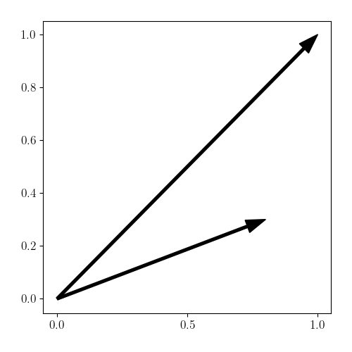
Suppose we now perform a Nyström approximation with rank $m=1$, and let’s use $x_1$ as our representative point. Plugging in our data to Equation \ref{eq:K22}, we can obtain an approximation for $K_{22}$:

\begin{align} K_{22} &= x_2^\top x_1 \frac{x_1^\top}{\sqrt{x_1^\top x_1}} \frac{1}{x_1^\top x_1} \frac{x_1}{\sqrt{x_1^\top x_1}} x_1^\top x_2 \\ &= x_2^\top x_1 \frac{x_1^\top x_1}{(x_1^\top x_1)^2} x_1^\top x_2. \\ \end{align}

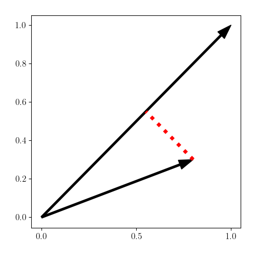
We can notice that this is identical to first projecting $x_2$ onto $x_1$ and then computing the covariance. To see this, note that the projection onto $x_1$ is given by

Computing the (linear) covariance then gives us

\begin{align} K_{22} &= \frac{x_2^\top x_1}{\|x_1\|^2} x_1^\top x_1 \frac{x_2^\top x_1}{\|x_1\|^2} \\ &= x_2^\top x_1 \frac{x_1^\top x_1}{(x_1^\top x_1)^2} x_1^\top x_2. \end{align}

We can visualize this projection below (in the red dotted line). Once the vector has been projected, the covariance can be computed along the representative vector.

Time complexity

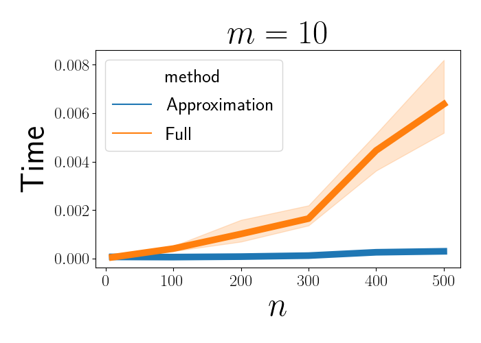
As mentioned above, one of the primary advantages of the Nyström approximation is the boost it gives in time performance for many algorithms. To demonstrate this, here we perform a simulation where we compute the time required to compute a matrix inverse using two methods: 1) inverting a full covariance matrix, and 2) approximating the inverse by first performing a Nyström approximation.

The code to perform this experiment is below:

import numpy as np
import time

n_list = [10, 100, 200, 300, 400, 500]
n_repeats = 5
p = 5
m = 10

kernel = lambda x1, x2: x1 @ x2.T
full_times = np.zeros((n_repeats, len(n_list)))
approx_times = np.zeros((n_repeats, len(n_list)))

for ii in range(n_repeats):
    for jj, n in enumerate(n_list):

        X = np.random.normal(size=(n, p))
        Xtilde = np.random.normal(size=(m, p))

        K_full = kernel(X, X)

        start = time.time()
        np.linalg.inv(K_full + 1e-10 * np.eye(n))
        end = time.time()
        full_time = end - start
        full_times[ii, jj] = full_time

        K11 = kernel(Xtilde, Xtilde)
        Lam, U = np.linalg.eigh(K11)
        K21 = X @ Xtilde.T
        K_approx = K21 @ U @ np.diag(1 / Lam) @ U.T @ K21.T

        start = time.time()
        left_term = K21 @ U
        middle_term = np.linalg.inv(Lam + U.T @ K21.T @ K21 @ U + 1e-10 * np.eye(m))
        left_term @ middle_term @ left_term.T
        end = time.time()
        approx_time = end - start
        approx_times[ii, jj] = approx_time

We can then plot the time required to invert the full matrix and the approximate matrix. Below, we see that as $n$ increases, the inversion of the full matrix increases rapidly, at a rate of approximately $n^3$.

References

• Rasmussen, Carl Edward. “Gaussian processes in machine learning.” Summer school on machine learning. Springer, Berlin, Heidelberg, 2003.
• Liu, Haitao, et al. “When Gaussian process meets big data: A review of scalable GPs.” IEEE transactions on neural networks and learning systems 31.11 (2020): 4405-4423.
• This stackoverflow post.