Normalizing flows

\(\DeclareMathOperator*{\argmin}{arg\,min}\) \(\DeclareMathOperator*{\argmax}{arg\,max}\)

Normalizing flows are a family of methods for flexibly approximating complex distributions. By combining ideas from probability theory, statistics, and deep learning, the learned distributions can be much more complex than traditional approaches to density estimation.

Motivation

In the field of approximate inference, we are interested in understanding some complex distribution (typically a posterior $p(z | x)$) whose density can’t be solved for analytically. A common approach is to approximate this posterior with a family of nice, tractable distributions.

A common choice for this approximate (or “variational”) family is a mean-field Gaussian distribution. Although mean-field Gaussians are convenient to work with mathematically, their expressive power is limited. For example, this class of distributions is be unable to capture the multiple peaks of a multimodal distribution. Thus, there’s a need for methods that allow for more complex approximate distributions while also maintaining computational tractability.

This is where normalizing flows come into play. By starting with a simple approximate distribution, and then passing it through a sequence of invertible transformations, we can end up with a complex resulting distribution.

Below, we first review variational autoencoders (another family of methods that is related but distinct), and then we describe normalizing flows.

Variational autoencoder

Recall the variational autoencoder (VAE) approach to inference. We again have a posterior density $p(z | x)$ that is intractble. A generic variational inference approach would posit a variational family of distributions $\mathcal{Q}_\phi$ with parameter $\phi$, and find the distribution $q_{\phi^\star}(z) \in \mathcal{Q}$ that best approximates the true posterior. In particular, $q$ is often assumed to be a set of mean-field Gaussians, $q(z) = \prod\limits_{k=1}^K \mathcal{N}(z_k | \mu_k, \sigma_k^2 I)$.

The key distinguishing feature of a VAE is that it parameterizes the variational parameters using a neural network. The inputs to this neural network are the data $x$. In particular, the variational generative process is given by

\begin{align} z_k &\sim \mathcal{N}(\mu_k, \sigma_k^2 I) \\ \mu_k &= [f(x)]_k \end{align}

where $f$ is a multi-output neural network. This allows the parameters $\{(\mu_k, \sigma^2_k)\}_{k=1}^K$ of the approximate posterior to be complex functions of the input.

However, a key limitation of VAEs is that, although the neural network parameterization is quite flexible, the final variational distribution is still a simple isotropic Gaussian (or another simple distribution). These classes are typically not flexible enough to capture complex posteriors. Normalizing flows seek to solve this issue.

Normalizing flows

Normalizing flows take inspiration from VAEs, but allow for much more flexible approximate posteriors. Rather than passing the (fixed) input through a neural network, normalizing flows transform the distribution itself with a complex function (like a neural network).

Suppose that $z$ is a random variable with PDF $p(z)$ and we take $z^\prime$ to be a transformation of $z$ such that $z^\prime = f(z)$. Recall that if $f$ has some nice properties, we can compute the density of $z^\prime$ with a simple formula that accounts for the change in volume induced by the transformation. This formula is given by

The benefit of doing this is that we can work with the new, transformed density that will be more flexible than the initial one. Furthermore, if we can parameterize $f$ with a flexible class of functions, we can tweak the function’s parameters to get different types of distributions. Notice that, unlike a VAE, we’re not just assuming some functional form for the parameters of the variational distribution. Rather, we’re parameterizing the entire density function.

Performing variational inference with noramlizing flows uses this exact principle: use a transformation to get a complex approximating distribution that still has a closed-form density function. Furthermore, we don’t have to limit ourselves to just one transformation. We can actually string together a sequence of transformations to get ever-more complex distributions.

Concretely, suppose we have an initial random variable $z_0$ that comes from a simple distribution $q_0$ (think, e.g., mean-field Gaussian). Further, suppose we have $K$ transformation functions $f_1, \dots, f_K$. By composing these functions together, we get a “flow” of transformations:

where we use the “open circle” notation to denote $f_i \circ f_j(x) = f_i(f_j(x))$.

And this is the complete fundamental idea: transformations on transformations.

Below, we’ll take a short detour to explore the intuition behind transforming random variables, and then we’ll return to explain how normalizing flows are used in variational inference.

Transformation of random variables

To understand the transformation of random variables more intuitively, let’s consider a couple simple examples.

Example: linear transformation of a Uniform RV

Let $z \sim \text{Unif}(0, 1)$ and suppose we linearly scale $z$ such that $z^\prime = f(z) = 3z$. We have $p(z) = 1$. The first thing that we can notice is that the support of $z^\prime$ will be different than $z$. While $z$ was always between $0$ and $1$, $z^\prime$ will range from $0$ to $3$.

Applying the above formula, we have

\begin{align} p(z^\prime) &= p(\frac13 z^\prime) \cdot \frac13 \\ &= 1 \cdot \frac13 \\ &= \frac13. \end{align}

Thus, this affine transformation of a uniform random variable results in a “squashing” of the PDF, as seen in the plot below.

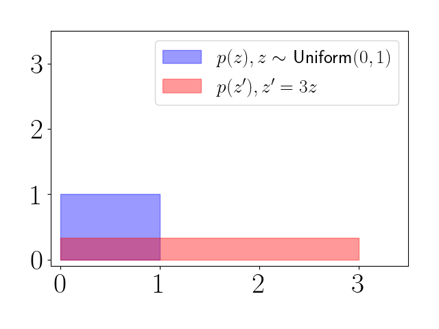
The transformation equation above is meant to account for the volume change in certain regions of space following the transformation. This is what’s happening with the red density: it must flatten and stretch to accomodate the density in the range $[0, 3]$.

Example: quadratic transformation of a Uniform RV

Let’s consider a slightly more interesting example. Let $z \sim \text{Unif}(0, 1)$ again and this time let $z^\prime = f(z) = z^2$. Again, applying the above formula, we have

\begin{align} p(z^\prime) &= p(\sqrt{z^\prime}) \cdot \frac{1}{2z^\prime} \\ &= 1 \cdot \frac{1}{2z^\prime} \\ &= \frac{1}{2z^\prime}. \end{align}

Clearly, the resulting random variable is no longer uniformly distributed. Instead, the density looks like the red plot below. (We’ve truncated the y-axis at $5$ here.)

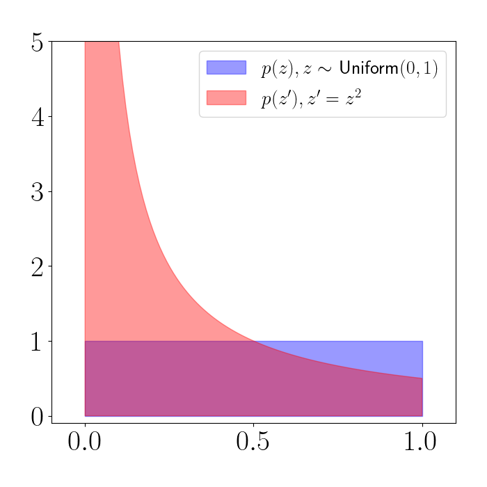
We can see that the density is being squashed toward $0$. In other words, regions of the support of $z$ are shifting their density downward in the density of $z^\prime$.

To see this, consider the plot below. The yellow and green regions represent a particular set of volumes in each density (the regions $[0.1, 0.3]$ and $[0.7, 0.9]$). On the left, each of these volumes is a rectangle in the uniform density. After the transformation on the right, we see that the yellow volume gets squished into a very narrow and tall part of the density near zero, while the green density gets expanded.

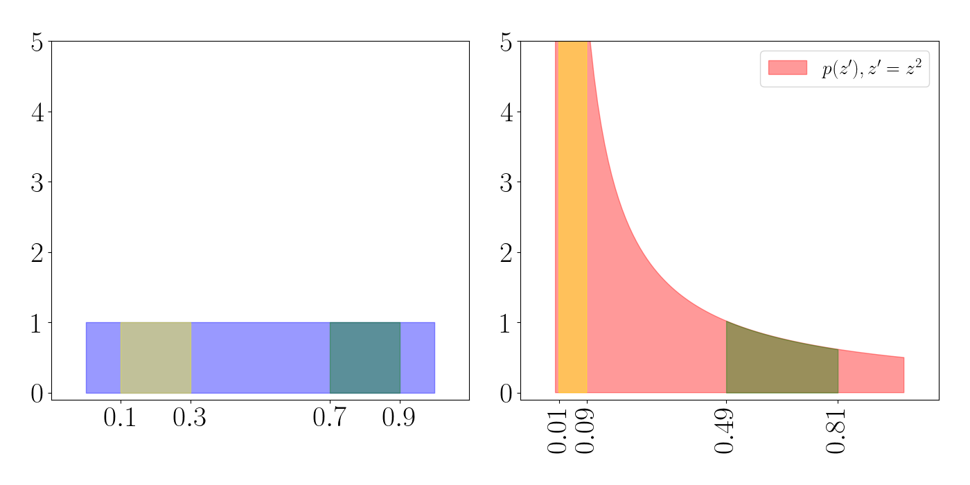
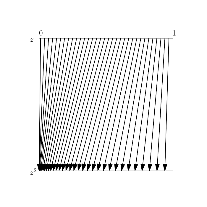
These expansions and contractions are what’s accounted for in the equation for the density of a transformed random variable. To see this one other way, consider the plot below. Here, we choose a subset of the support of $z$ and show where these map to in $z^\prime$ (represented by each arrow). We can see that the density is contracting near $0$, and expanding as we move toward $1$.

Example: linear transformation of a Gaussian RV

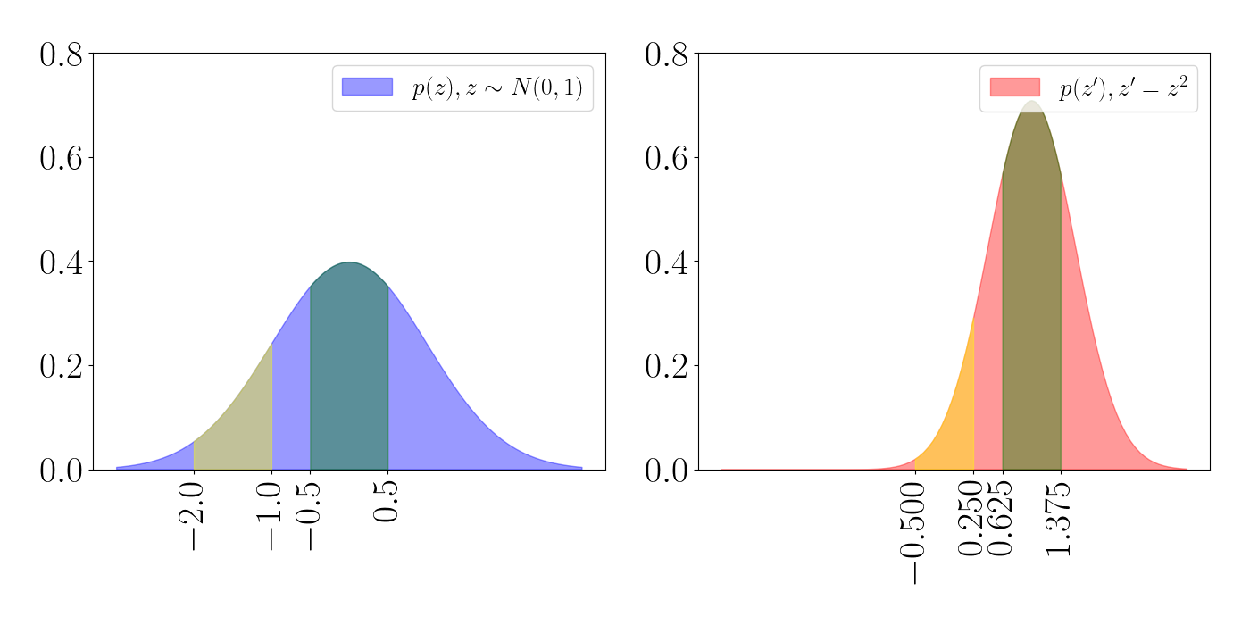
Finally, let’s consider a non-uniform example: a linear transformation of a univariate Gaussian random variable. In particular, assume

where $w \in \mathbb{R}$ and $b \in \mathbb{R}$ is some scalar weight and translation parameter, respectively.

Then using the above formula, we have

\begin{align} p(z^\prime) &= p(\frac1w (z^\prime - b)) \cdot \frac{1}{w} \\ &= \frac{1}{\sqrt{2\pi \sigma^2}} \exp\left\{ \frac{1}{2\sigma^2} (\frac1w (z^\prime - b) - \mu)^2 \right\} \cdot \frac1w \\ &= \frac{1}{\sqrt{2\pi \sigma^2}} \exp\left\{ \frac{1}{2\sigma^2} (\frac{1}{w^2} (z^\prime - b)^2 - 2 \frac{1}{w} (z^\prime - b) \mu + \mu^2) \right\} \cdot \frac1w \\ &= \frac{1}{\sqrt{2\pi \sigma^2}} \exp\left\{ \frac{1}{2\sigma^2} (\frac{1}{w^2} (z^{\prime 2} - 2z^\prime b + b^2) - 2 \frac{1}{w} (z^\prime \mu - b \mu) + \mu^2) \right\} \cdot \frac1w \\ &= \frac{1}{\sqrt{2\pi \sigma^2}} \exp\left\{ \frac{1}{2\sigma^2 w^2} ((z^{\prime 2} - 2z^\prime b + b^2) - 2 w (z^\prime \mu - b \mu) + w^2 \mu^2) \right\} \cdot \frac1w \\ &= \frac{1}{\sqrt{2\pi \sigma^2 w^2}} \exp\left\{ \frac{1}{2\sigma^2 w^2} (z^\prime - (w \mu + b))^2 \right\}. \end{align}

We can see that the last line is a Gaussian PDF and conclude that

Consider the case when $w=0.75, b=1$. We can again track the volume changes with a similar plot as above:

Inference with normalizing flows

Similar to VAEs, our goal during inference using normalizing flows is to optimize the parameters of the transformation funciton $f$ such that the approximate posterior is “close” to the true posterior. In particular, we can think about the parameters $\phi$ of the transformation function as the variational parameters, and maximize the ELBO with respect to $\phi$. Recall that the ELBO $\mathcal{L}$ is given by

We can get an unbiased approximation of the ELBO using Monte Carlo samples,

In vanilla variational inference, we would parameterize $q$ as a specific family of distributions. In the case of normalizing flows, we think of $q$ as a transformed random variable, with initial distribution $q_0(z)$. Thus, the sampling process will consist of one sampling step from $q_0$ followed by a composition of functions.

Importantly, notice that we can evaluate the final variational density $q_K(z)$ because we can actually compute its density function.

We can then easily carry out inference using gradient-based optimization. As long as we can compute the gradient of the cost function with respect to the variational parameters, we’re good to go. The algorithm for performing variational inference with normalizing flows is then as follows.

1. While ELBO has not converged:
   1. Sample $S$ base random variables $z_{s0} \sim q_0(z)$ for $s=1, \dots, S$.
   2. Pass each sample through the transformation functions $z_s = f_K \circ f_{K-1} \circ \cdots \circ f_1(z_{s0})$.
   3. Using these transformed samples, compute an estimate of the gradient of the ELBO w.r.t. the variational parameters, $\widetilde{\nabla}_{\phi}\mathcal{L}$.
   4. Update the variational parameters using gradient ascent or some other optimization procedure, $\phi = \phi + \widetilde{\nabla}_{\phi}\mathcal{L}$.

Example

Consider a simple example: a linear transformation of a Guassian. Let $z_0 \sim \mathcal{N}(0, I)$. Then our function is:

where $A$ is a $2 \times 2$ matrix and $b$ is a $2$-vectors of biases. Clearly, the resulting distribution is $z_K \sim \mathcal{N}(b, AA^\top)$. (Note that in this case, we could have directly parameterized the approximate distribution, but we take the normalizing flow perspective for didactic reasons.)

Our goal is then to find the $A$ and $b$ that maximize the ELBO. Below is a simple example of doing so in Python.

from __future__ import absolute_import
from __future__ import print_function
import matplotlib.pyplot as plt

import autograd.numpy as np
import autograd.numpy.random as npr
import autograd.scipy.stats.multivariate_normal as mvn
import autograd.scipy.stats.norm as norm

from autograd import grad
from autograd.misc.optimizers import adam


def black_box_variational_inference(logprob, D, num_samples):
    """Implements http://arxiv.org/abs/1401.0118, and uses the
    local reparameterization trick from http://arxiv.org/abs/1506.02557"""

    def unpack_params(params):
        # Variational dist is a diagonal Gaussian.
        weights, bias = np.reshape(params[:D**2], (D, D)), params[D**2:]
        return weights, bias

    def gaussian_entropy(cov):
        return 0.5 * D * (1.0 + np.log(2*np.pi)) + np.linalg.slogdet(cov)[1]

    rs = npr.RandomState(0)
    def variational_objective(params, t):
        """Provides a stochastic estimate of the variational lower bound."""
        weights, bias = unpack_params(params)

        # *** We can explicitly write the distribution in terms of the parameters ***
        # (For a Gaussian, this is easy)
        mean, cov = bias, weights @ weights.T + 0.01 * np.eye(D)
        samples = rs.randn(num_samples, D) @ weights + bias
        lower_bound = gaussian_entropy(cov) + np.mean(logprob(samples, t))
        return -lower_bound

    gradient = grad(variational_objective)

    return variational_objective, gradient, unpack_params



if __name__ == '__main__':

    # Specify an inference problem by its unnormalized log-density.
    D = 2

    def log_density(x, t):
        return mvn.logpdf(x, np.zeros(D), np.array([[1, 0.4], [0.4, 1]]))

    # Build variational objective.
    objective, gradient, unpack_params = \
        black_box_variational_inference(log_density, D, num_samples=2000)

    # Set up plotting code
    def plot_isocontours(ax, func, xlimits=[-4, 4], ylimits=[-4, 4], numticks=101):
        x = np.linspace(*xlimits, num=numticks)
        y = np.linspace(*ylimits, num=numticks)
        X, Y = np.meshgrid(x, y)
        zs = func(np.concatenate([np.atleast_2d(X.ravel()), np.atleast_2d(Y.ravel())]).T)
        Z = zs.reshape(X.shape)
        plt.contour(X, Y, Z)
        ax.set_yticks([])
        ax.set_xticks([])

    # Set up figure.
    fig = plt.figure(figsize=(8,8), facecolor='white')
    ax = fig.add_subplot(111, frameon=False)
    plt.ion()
    plt.show(block=False)

    def callback(params, t, g):
        print("Iteration {} lower bound {}".format(t, -objective(params, t)))

        plt.cla()
        target_distribution = lambda x : np.exp(log_density(x, t))
        plot_isocontours(ax, target_distribution)

        weights, bias = unpack_params(params)
        cov = weights @ weights.T
        variational_contour = lambda x: mvn.pdf(x, bias, cov)
        plot_isocontours(ax, variational_contour)
        plt.draw()
        plt.pause(1.0/30.0)

    print("Optimizing variational parameters...")

    ## Initialize parameters of the transformation
    init_weights = np.random.normal(size=(D**2))
    init_bias    = -3 * np.random.normal(size=(D))
    init_var_params = np.concatenate([init_weights, init_bias])
    variational_params = adam(gradient, init_var_params, step_size=0.1, num_iters=2000, callback=callback)

References

• Rezende, Danilo, and Shakir Mohamed. “Variational inference with normalizing flows.” International conference on machine learning. PMLR, 2015.