Andy Jones
Nearest neighbor Gaussian processes
\(\DeclareMathOperator*{\argmin}{arg\,min}\) \(\DeclareMathOperator*{\argmax}{arg\,max}\)
Nearest neighbor Gaussian processes (NNGPs) are sparse and fast approximations for Gaussian process (GP) models. Here, we review the fundamental ideas behind the approach and show a simple simulation.
NNGPs have been especially popular in the geostatistical modeling community. Below, I will implicitly assume that we’re working with an input dimension of $D=2$ (corresponding to two spatial coordinates) unless noted otherwise, although all of these ideas can easily be generalized to problems of arbitrary dimension.
Nearest neighbor Gaussian process
Consider a set of $n$ observations from a zero-mean GP:
\[\mathbf{y} = (y_1, \cdots, y_n)^\top \sim \mathcal{N}(\mathbf{0}, \mathbf{K}_{\mathbf{X} \mathbf{X}})\]where $\mathbf{K}_{\mathbf{X} \mathbf{X}}$ is an $n \times n$ covariance matrix containing all evaluations of a kernel function $k(\cdot, \cdot)$ at all pairs of points.
Using basic rules of probability, we can equivalently express the distribution of $\mathbf{y}$ in terms of a set of conditional probabilities:
\begin{align} p(\mathbf{y}) = p(y_1, \dots, y_n) &= p(y_1) p(y_2 | y_1) \cdots p(y_n | y_1, \dots, y_{n - 1}) \\ &= p(y_1) \prod\limits_{i=2}^n p\left(y_i | \{y_j\}_{j=1}^{i-1}\right). \end{align}
We’ll see why expressing the joint density this way is useful in a moment.
Vecchia’s approximation
Each of the conditional densities above, $p\left(y_i | \{y_j\}_{j=1}^{i-1}\right)$, will depend on some number of other points. However, it’s useful to ask the question: do we really need to condition on all these other points, especially if they contain very little information about the point of interest? This is the key idea of the NNGP: to model our data, we often don’t need to model the influence between all pairs of points; instead we can just consider a few of each point’s “neighbors”.
In particular, consider approximating each of the conditional densities $p\left(y_i | \{y_j\}_{j=1}^{i-1}\right)$ by conditioning on just $m$ samples, where $m \ll n$. For a given sample $x_i$, we will call these $m$ samples the “neighbors” of $x_i$, which we will denote as $N(x_i)$. We then have the following approximation of $p(\mathbf{y})$:
\[\widetilde{p}(\mathbf{y}) = \prod\limits_{i=1}^n p(y_i | \mathbf{y}_{N(x_i)})\]where $\mathbf{y}_{N(x_i)}$ is the subvector of $\mathbf{y}$ containing all $y_j$ such that $x_j \in N(x_i)$. This approximation was originally proposed by Aldo Vecchia in 1988, and is now widely known as “Vecchia’s approximation”.
Choosing neighbors
A natural question that arises under this approximation is how to define each set of neighbors $N(\mathbf{x}_i)$. For our purposes, we need the ultimate model to be a valid probability distribution, so we are most interested in working with directed acyclic graphs (DAGs) (see the references at the bottom for a more detailed explanation).
In order to form a valid DAG, we’ll follow the following process. First, order the input points $\mathbf{x}_1, \dots, \mathbf{x}_n$ according to some criterion (e.g., sort them by their first coordinate). Next, define a valid distance metric between points (e.g., Euclidean distance). Finally for each element $i$, define the $m$ nearest neighbors $N(\mathbf{x}_i)$ to be the set of points $\mathbf{x}_{j_1}, \dots, \mathbf{x}_{j_m}$ such that all neighbor indices $j_1, \dots, j_m$ are less than $i$.
Let’s see a simple example. Consider the spatial coordinates below.
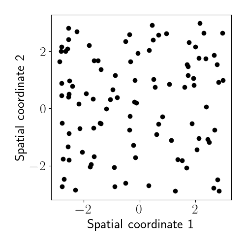
Let’s order these by their first coordinate and find their $m=10$ nearest neighbors according to the process above. Here’s an example of what the relationships look like for one point:
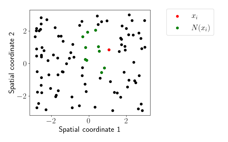
We can see that all neighboring points are to the “left” of $x_i$ due to our ordering based on the first spatial coordinate.
Let’s generalize these neighbor relationships across all points. Below is a heatmap of the neighbor relationships, with a white square indicating that sample $j$ is a neighbor of sample $i$, and a black square indicating no neighbor relationship.
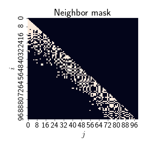
It’s worth noting that the neighbors will crucially depend on the choice of ordering of the points. While we chose one particular order of the points, many others could have been chosen. Interestingly (and luckily), several authors have pointed out that the model doesn’t seem to be particularly sensitive to the choice of ordering in most empirical findings.
Relevant densities for the NNGP
Given the nice properties of the multivariate Gaussian distribution, we can write out the mean and covariance of the $p(y_i | \mathbf{y}_{N(x_i)})$ terms explicitly. Their forms are given by the conditional distribution of a multivariate Gaussian. In particular, we have
\begin{align} y_i | \mathbf{y}_{N(\mathbf{x}_i)} &\sim \mathcal{N}(\mathbf{B}_{\mathbf{x}_i} \mathbf{y}_{N(\mathbf{x}_i)}, \mathbf{F}_{\mathbf{x}_i}) \\ \mathbf{B}_{\mathbf{x}_i} &= \mathbf{K}_{\mathbf{x}_i, N(\mathbf{x}_i)} \mathbf{K}_{N(\mathbf{x}_i)} \\ \mathbf{F}_{\mathbf{x}_i} &= \mathbf{K}_{\mathbf{x}_i} - \mathbf{K}_{\mathbf{x}_i, N(\mathbf{x}_i)} \mathbf{K}_{N(\mathbf{x}_i)}^{-1} (\mathbf{K}_{\mathbf{x}_i, N(\mathbf{x}_i)})^\top \\ \end{align}
We can now show that, given these individual conditional distributions, the joint distribution $\widetilde{p}(\mathbf{y})$ will be Gaussian with a sparse precision matrix. Focusing on the exponentiated part of the density for $\widetilde{p}$, we have
\begin{equation} \sum\limits_{i=1}^n (\mathbf{y}_i - \mathbf{B}_{\mathbf{x}_i} \mathbf{y}_{N(\mathbf{x}_i)})^\top \mathbf{F}_{\mathbf{x}_i}^{-1} (\mathbf{y}_i - \mathbf{B}_{\mathbf{x}_i} \mathbf{y}_{N(\mathbf{x}_i)}). \tag{1} \label{eq:inner_prod} \end{equation}
This term only accounts for the covariance between a point $\mathbf{x}_i$ and its neighbors $N(\mathbf{x}_i)$; however, we will want to form the full $n \times n$ covariance matrix. To do this, let’s first write down the contribution of each sample $\mathbf{x}_j$ to the term $\mathbf{B}_{\mathbf{x}_i}$. Note that for most samples (those that aren’t neighbors to $\mathbf{x}_i$), this contribution will be zero. In particular, we have three cases:
\[b_{\mathbf{x}_i, \mathbf{x}_j}^\star = \begin{cases} 1, & i=j \\\ \mathbf{B}_{\mathbf{x}_i}[\ell], & \mathbf{x}_j = N(\mathbf{x}_j)[\ell] \text{ for some } \ell \\\ 0, & \text{otherwise.} \end{cases}\]Now let $\mathbf{B}^\star_{\mathbf{x}_i}$ be the vector containing all of these elements for sample $i$,
\[\mathbf{B}^\star_{\mathbf{x}_i} = (b_{\mathbf{x}_i, \mathbf{x}_1}^\star, \cdots, b_{\mathbf{x}_i, \mathbf{x}_n}^\star)^\top.\]Note that each of these vectors will have at most $m + 1$ nonzero entries.
Furthermore, we can stack each of these vectors together into an $n \times n$ matrix,
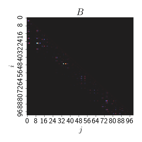
\[\mathbf{B} = ((\mathbf{B}^\star_{\mathbf{x}_1})^\top, \dots, (\mathbf{B}^\star_{\mathbf{x}_n})^\top)^\top.\]At this point, we can notice that $\mathbf{B}$ will be a lower triangular matrix. It will also be sparse due to our assumption that $m \ll n$. Below is a heatmap of $\mathbf{B}$ for our synthetic data.
Likewise, let’s define $\mathbf{F}$ to be an $n \times n$ diagonal matrix:
\[\mathbf{F} = diag(\mathbf{F}_{\mathbf{x}_1}, \dots, \mathbf{F}_{\mathbf{x}_n})\]Using these new matrices, we can then rewrite Equation \eqref{eq:inner_prod} as
\[\sum\limits_{i=1}^n \mathbf{y}^\top (\mathbf{B}_{\mathbf{x}_i}^\star)^\top \mathbf{F}_{\mathbf{x}_i}^{-1} \mathbf{B}_{\mathbf{x}_i}^\star \mathbf{y} = \mathbf{y}^\top \mathbf{B}^\top \mathbf{F}^{-1} \mathbf{B} \mathbf{y}.\]This implies that the precision matrix of $\widetilde{p}(\mathbf{y})$ is given by
\[\widetilde{\Sigma}^{-1} = \mathbf{B}^\top \mathbf{F}^{-1} \mathbf{B}.\]Altogether, these properties imply both a sparse precision matrix $\widetilde{\Sigma}^{-1}$ and a sparse covariance matrix $\widetilde{\Sigma}$. Below, we plot the covariance matrix for a full GP (left) and the covariance matrix for the NNGP (right).
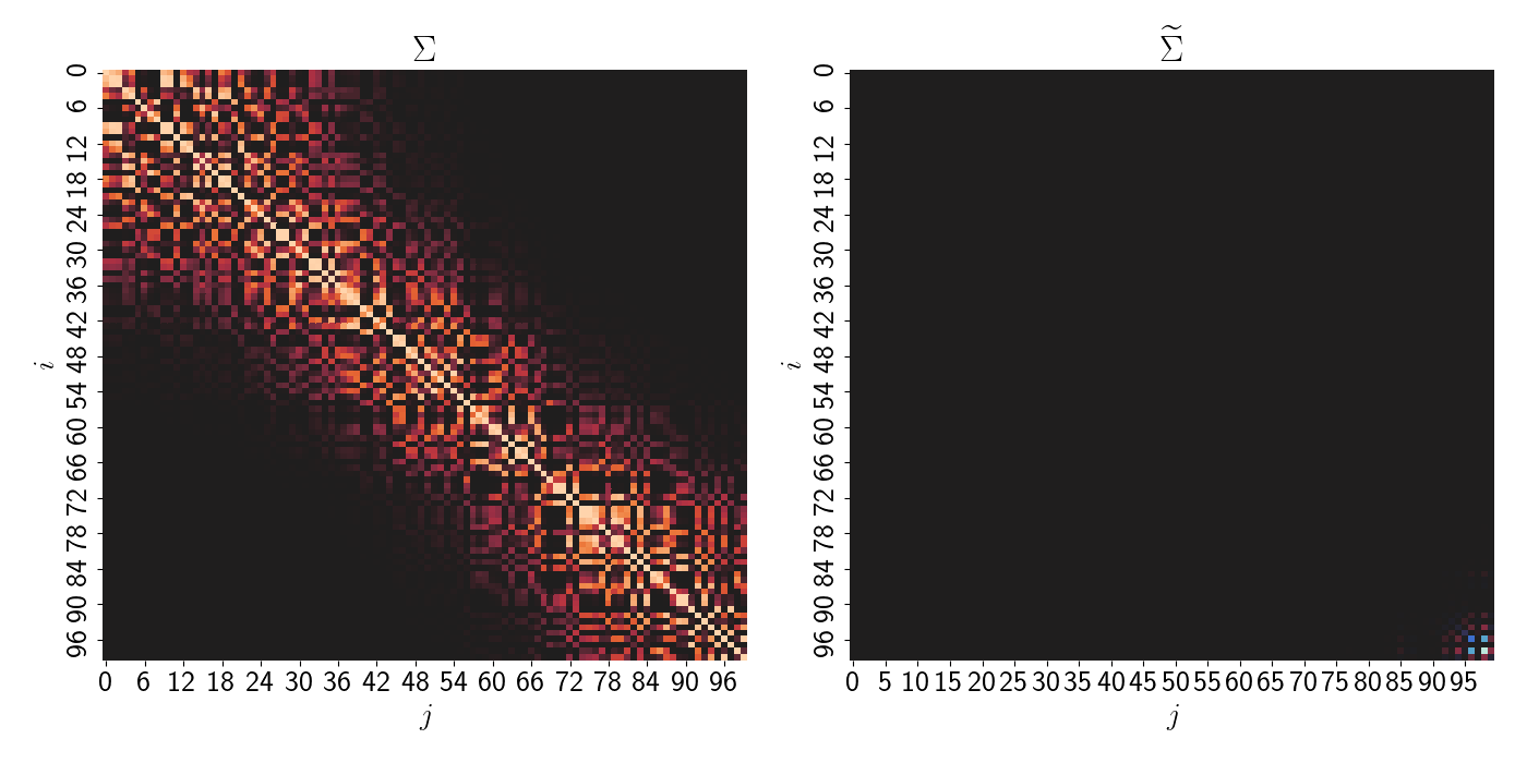
The forms of the precision and covariance matrices start to make the computational benefits of the NNGP clear. First of all, we avoid the need to invert a large ($n \times n$) matrix. Instead, we only have to invert $\mathbf{F}$, which is trivial because it’s diagonal.
Second, the determinant of $\widetilde{\Sigma}$ will be easy to calculate. Recall that the determinant of a triangular matrix is equal to the product of its diagonal elements. In the NNGP, this implies that $det(\mathbf{B}) = 1$. Thus, using other basic properties of determinants, the determinant of $\widetilde{\Sigma}$ is given by
\begin{align} det(\widetilde{\Sigma}) &= det((\mathbf{B}^\top \mathbf{F}^{-1} \mathbf{B})^{-1}) \\ &= \frac{1}{det(\mathbf{B}^\top \mathbf{F}^{-1} \mathbf{B})} & \left( det(\mathbf{A}^{-1}) = 1/det(\mathbf{A}) \right) \\ &= \frac{1}{det(\mathbf{B}^\top) det(\mathbf{F}^{-1}) det(\mathbf{B})} & \left( det(\mathbf{A} \mathbf{C}) = det(\mathbf{A}) det(\mathbf{C}) \right) \\ &= \frac{1}{1 \cdot det(\mathbf{F}^{-1}) \cdot 1} \\ &= det(\mathbf{F}) \\ &= \prod\limits_{i=1}^n \mathbf{F}_{\mathbf{x}_i} & \left(det(diag(a_1, \dots, a_K)) = \prod_k a_k\right). \end{align}
The determinant can be computed in linear time by taking the product of the diagonal elements of $\mathbf{F}$.
Predictions
We can easily make predictions under the NNGP model using the same ideas as above. Suppose we have a set of $k$ test input points $\mathbf{x}_1^\star, \dots, \mathbf{x}_K^\star$. Then simply using the conditional distribution for the multivariate normal, we can obtain the predictive mean:
\[\mu_k^\star = \mathbf{B}_{\mathbf{x}_k^\star} \mathbf{y}_{N(\mathbf{x}_k^\star)}.\]Here, $\mathbf{B}_{\mathbf{x}_k^\star}$ is defined analogously to $\mathbf{B}_{\mathbf{x}_i}$ but using the neighbors of $\mathbf{x}_k^\star$ in the training data.
Let’s see a simple example. Here, let’s consider one-dimensional inputs for visual clarity. Below, we plot the predictions from the NNGP with $m=10$ in red, and the predictions from a full GP in green. The data is are the black points.
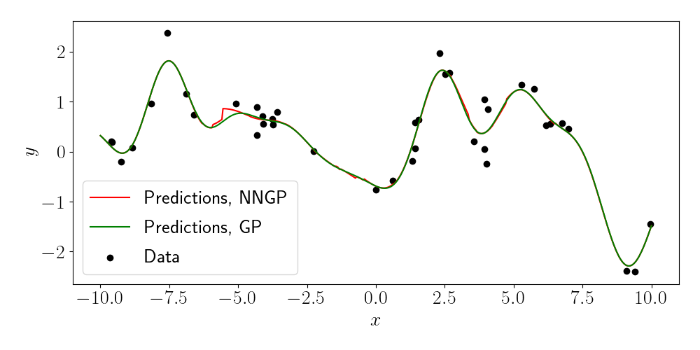
We can see that, although the NNGP predictions deviate from the full GP in some places, they are overall quite similar. We can also examine what happens as we vary the number of neighbors $m$ (as indicated in the title of each plot).
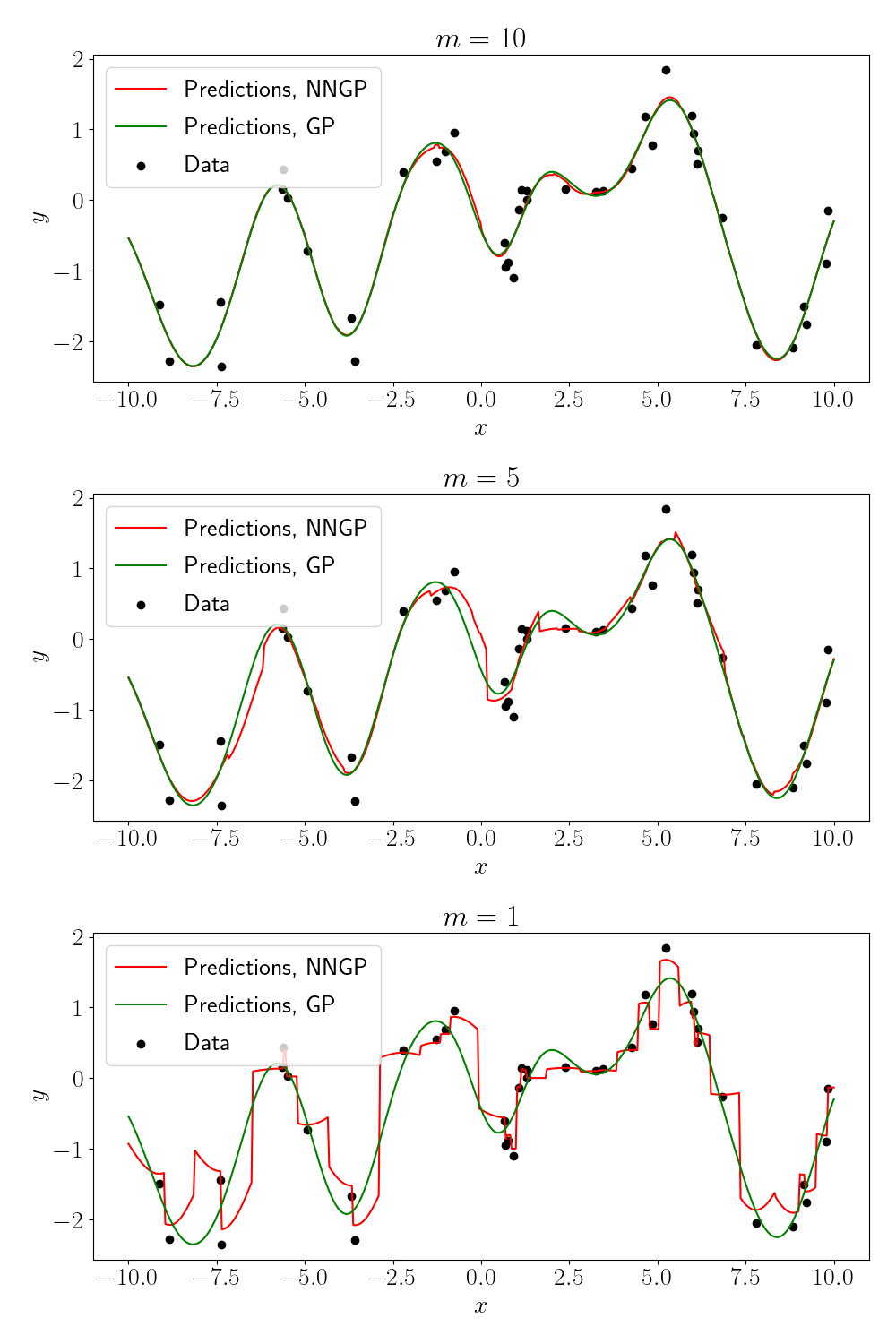
As we might expect, when there is only $1$ neighbor for each point, the predictions essentially predict the value of the neighbor itself.
Code
Code for the simulations above can be found in this GitHub repository. Note that the code here is only meant for simple demonstrations, and more robust NNGP codebases should be used for real applications.
References
- Datta, Abhirup, et al. “Hierarchical nearest-neighbor Gaussian process models for large geostatistical datasets.” Journal of the American Statistical Association 111.514 (2016): 800-812.
- Vecchia, Aldo V. “Estimation and model identification for continuous spatial processes.” Journal of the Royal Statistical Society: Series B (Methodological) 50.2 (1988): 297-312.
- Lu Zhang’s blog post on NNGPs in Stan.