Neural networks as Gaussian processes

\(\DeclareMathOperator*{\argmin}{arg\,min}\) \(\DeclareMathOperator*{\argmax}{arg\,max}\)

Neural networks effectively, become equivalent to Gaussian processes as the number of hidden units tends to infinity. Below, we explore this relationship. First, we define the problem setup, and then we show how the function represented by a neural network of infinite width is a draw from a Gaussian process.

The network

Suppose we have a set of inputs $\mathbf{x}_i \in \mathbb{R}^D$ and corresponding outputs $y_i \in \mathbb{R}$ for $i = 1, \dots, n$. Let’s construct a simple neural network with one hidden layer. Assume that there are $H$ hidden units and each unit has an identical element-wise nonlinearity $g(\cdot)$. The functional form of a neural network with one hidden layer can be written as follows.

\begin{align} f(\mathbf{x}_i) &= \mathbf{w}_2^\top \mathbf{h}_i + b_2 \\ \mathbf{h}_i &= g(\mathbf{W}_1 \mathbf{x}_i + \mathbf{b}_1). \end{align}

where $\mathbf{h}_i \in \mathbb{R}^H$ is a vector of the outputs of the hidden units, $\mathbf{W}_1 \in \mathbb{R}^{H \times D}$ and $\mathbf{w}_2 \in \mathbb{R}^{H}$ are network weights, and $\mathbf{b}_1 \in \mathbb{R}^{H}$ and $b_2 \in \mathbb{R}$ are intercept terms.

Throughout this post, we’ll assume that the weights and biases are each i.i.d. draws from some mean-zero distributions with variances $\sigma^2_{\mathbf{W}_1}$, $\sigma^2_{\mathbf{w}_2}$, $\sigma^2_{\mathbf{b}_1}$, and $\sigma^2_{b_2}$.

Gaussian outputs

Note that we can rewrite the network output as a summation over the contribution from each hidden node:

Each of the terms in the summation will be independent and identically distributed due to our assumption of the initial distributions of the weights. Thus, by the central limit theorem, we know that $f(\mathbf{x}_i)$ will converge to a Gausisan distribution as $H \to \infty$. Furthermore, given a set of outputs $f(\mathbf{x}_1), f(\mathbf{x}_2), \dots, f(\mathbf{x}_n)$ based on distinct inputs, these will jointly follow a multivariate normal distribution as $H \to \infty$:

Thus, as its number of hidden units approaches infinity, a neural network with i.i.d. randomly-drawn parameters represents a function that is drawn from a Guassian process with covariance matrix $\mathbf{K}$.

Below, we show how to compute $\boldsymbol{\mu}$ and $\mathbf{K}$.

Mean and covariance

Let’s now inspect the mean of the network output and covariance between two arbitrary outputs. Let $\theta = \{\mathbf{W}_1, \mathbf{w}_2, \mathbf{b}_1, b_2\}$ be the set of network parameters.

First, let’s compute the mean.

To compute the covariance, let’s start from scratch and write out the basic definition of covariance, and expand terms.

\begin{align} \mathbb{E}_\theta[f(\mathbf{x}_i) f(\mathbf{x}_j)] &= \mathbb{E}_\theta[(\mathbf{w}_2^\top \mathbf{h}_i + b_2) (\mathbf{w}_2^\top \mathbf{h}_j + b_2)] \\ &= \mathbb{E}_{\theta}[(\mathbf{w}_2^\top \mathbf{h}_i) (\mathbf{w}_2^\top \mathbf{h}_j)] + \mathbb{E}_{\theta}[(\mathbf{w}_2^\top \mathbf{h}_i) b_2] \\ & ~~~~~~ + \mathbb{E}_{\theta}[(\mathbf{w}_2^\top \mathbf{h}_j) b_2] + \mathbb{E}_{\theta}[b_2^2]. \end{align}

We can split out each expectation into expectations over the relevant parameters and begin to simplify terms:

\begin{align} &\mathbb{E}_{\mathbf{W}_1, \mathbf{b}_1, \mathbf{w}_2}[(\mathbf{w}_2^\top \mathbf{h}_i) (\mathbf{w}_2^\top \mathbf{h}_j)] + \mathbb{E}_{\mathbf{W}_1, \mathbf{b}_1, \mathbf{w}_2}[(\mathbf{w}_2^\top \mathbf{h}_i)] \underbrace{\mathbb{E}_{b_2}[b_2]}_{0} \\ & ~~~~~~+ \mathbb{E}_{\mathbf{W}_1, \mathbf{b}_1, \mathbf{w}_2}[(\mathbf{w}_2^\top \mathbf{h}_j)] \underbrace{\mathbb{E}_{b_2}[b_2]}_{0} + \underbrace{\mathbb{E}_{b_2}[b_2^2]}_{\sigma^2_b} \\ =& \mathbb{E}_{\mathbf{W}_1, \mathbf{b}_1, \mathbf{w}_2}[(\mathbf{w}_2^\top \mathbf{h}_i) (\mathbf{w}_2^\top \mathbf{h}_j)] + \sigma^2_b. \end{align}

Finally, let’s expand the inner products, which will further simplify the covariance:

Because the parameters for each hidden unit are independent of one another, the expectation of all cross terms (between hidden units) will be zero. Thus, our covariance simplifies as

\begin{align} & \mathbb{E}_{\mathbf{W}_1, \mathbf{b}_1, \mathbf{w}_2}\left[\left(\sum\limits_{k=1}^H w_{2k}^2\right) \left(\sum\limits_{k=1}^H h_{ik} h_{jk} \right)\right] + \sigma^2_b \\ & \left(\sum\limits_{k=1}^H \mathbb{E}_{\mathbf{w}_2} [w_{2k}^2]\right) \mathbb{E}_{\mathbf{W}_1, \mathbf{b}_1}\left[\left(\sum\limits_{k=1}^H h_{ik} h_{jk} \right)\right] + \sigma^2_b \\ =& H\sigma^2_{\mathbf{w}_2}\mathbb{E}_{\mathbf{W}_1, \mathbf{b}_1}\left[\sum\limits_{k=1}^H h_{ik} h_{jk} \right] + \sigma^2_b. \end{align}

This final form implies that the covariance function imposed by a given network will depend on the activation function $g(\cdot)$, as well as the prior distributions on the input-to-hidden parameters, $\mathbf{W}_1, \mathbf{b}_1.$ Several closed-form covariance functions have been derived for specific settings of $g(\cdot)$ and the prior distributions (see the References for some examples).

Example

Consider a neural network with one hidden layer with a hyperbolic tangent (tanh) activation function.

def nn(X, n_hidden):
      W1 = np.random.normal(scale=10, size=(1, n_hidden))
      b1 = np.random.normal(scale=10, size=(1, n_hidden))
      W2 = np.random.normal(scale=1/np.sqrt(n_hidden), size=(n_hidden, 1))
      b2 = np.random.normal(scale=1, size=(1, 1))

      hidden_activations = np.tanh(X @ W1 + b1)
      output = hidden_activations @ W2 + b2
      return output

We plot example draws from this network with different values of $H$ below.

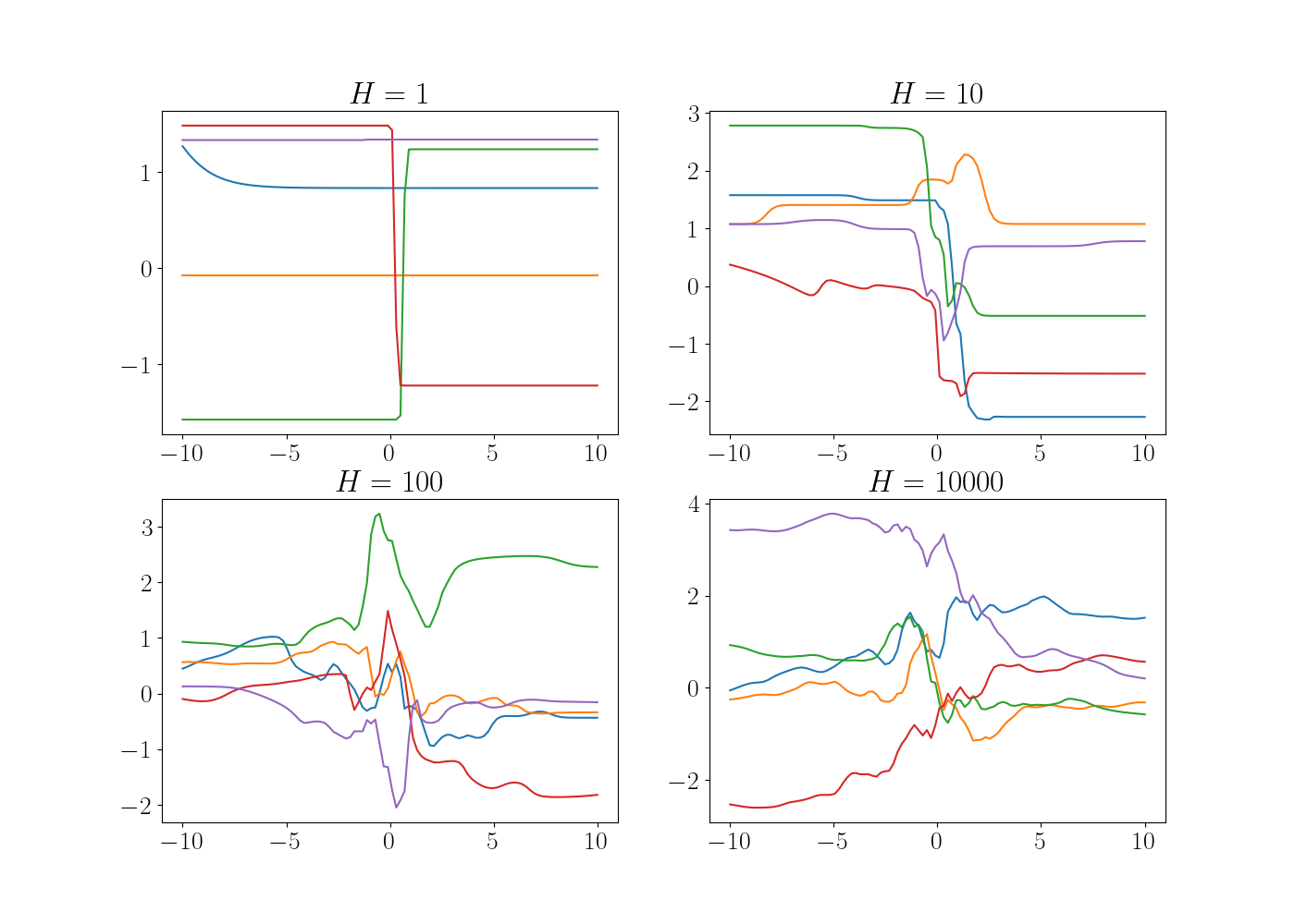
As expected, we can see that the sampled functions become more complex as the number of hidden units increases.

References

• Neal, Radford M. “Priors for infinite networks.” Bayesian Learning for Neural Networks. Springer, New York, NY, 1996. 29-53.
• Lee, Jaehoon, et al. “Deep neural networks as gaussian processes.” arXiv preprint arXiv:1711.00165 (2017).
• Williams, Christopher KI. “Computing with infinite networks.” Advances in neural information processing systems (1997): 295-301.
• Cho, Youngmin. Kernel methods for deep learning. University of California, San Diego, 2012.