Moment-generating functions

\(\DeclareMathOperator*{\argmin}{arg\,min}\) \(\DeclareMathOperator*{\argmax}{arg\,max}\)

While probability distributions are most commonly defined by their probability density functions (PDFs) and cumulative density functions (CDFs), there exist other characterizations as well. One of those is the moment-generating function, which we explore in this post.

Defining moment-generating functions

Consider a random variable $X.$ Its moment-generating function (MGF) is defined by

\begin{equation} M_X(t) = \mathbb{E}\left[e^{tX}\right]. \label{eq:mgf} \tag{1} \end{equation}

A key property of the MGF – and the one that gives the function its name – is that its derivatives with respect to $t$ are equal to the distribution’s moments. In other words, by differentiating the MGF w.r.t. $t,$ we “generate” the distribution’s moments.

To see this property, it is instructive to inspect the Taylor expansion of the MGF around $t=0$:

\begin{align} M_X(t) &= M_X(0) + t M_X^\prime(t) + \frac{1}{2!} t^2 M_X^{\prime\prime}(t) + \frac{1}{3!} t^3 M_X^{\prime\prime\prime}(t) + \cdots \\ &= \mathbb{E}\left[e^{0X}\right] + \mathbb{E}\left[t X e^{0X}\right] + \frac{1}{2!} \mathbb{E}\left[t^2 X^2 e^{0X}\right] + \frac{1}{3!} \mathbb{E}\left[t^3 X^3 e^{0X}\right] + \cdots \\ &= 1 + t \mathbb{E}[X] + \frac{1}{2!} t^2 \mathbb{E}[X^2] + \frac{1}{3!} t^3 \mathbb{E}[X^3] + \cdots, \end{align}

where we have used the fact that all derivatives of $e^t$ with respect to $t$ are equal to $e^t$ and the fact that $t$ can be removed from the expectation.

We can now clearly see that the $n$th derivative of the MGF with respect to $t$ evaluated at $t=0$ is equal to the $n$th moment.

\begin{align} m_0 &= 1 \\ m_1 &= \mathbb{E}[X] \\ m_2 &= \mathbb{E}[X^2] \\ m_3 &= \mathbb{E}[X^3] \\ &\vdots \end{align}

Importantly, recall that these moments are in general not the same as the distribution’s central moments (mean, variance, skew, etc.). Recall that the $n$th central moment is given by:

Of course, when $\mathbb{E}[X] = 0,$ then the moments and central moments coincide, but this will not be true in general.

We now demonstrate the MGF through a series of examples.

Example: Discrete distribution

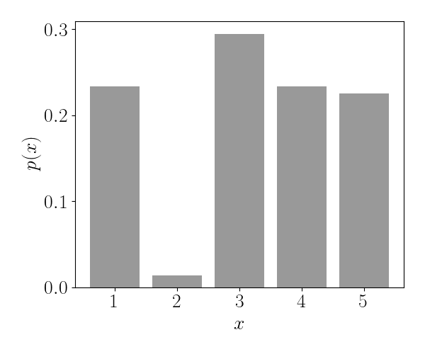
Consider a random variable $X$ drawn from a discrete probability distribution across $K$ states, where the probability of state $k$ is denoted as $p_k.$ The code and plot below shows an example with $K=5$ states.

import numpy as np
np.random.seed(2)
K = 5
states = np.arange(1, K + 1)
ps = np.random.uniform(size=K)
ps = ps / ps.sum()
plt.bar(states, ps)
plt.show()

In this case, the MGF is relatively straightforward to calculate by directly plugging into Equation \ref{eq:mgf}:

If the distribution is uniform (i.e., $p_1 = p_2 = \cdots = p_K = 1/K$), then the MGF can be further simplified as a geometric series.

Let’s visualize the MGF for the example discrete distribution above with $K=5$ states. Below we plot $M_X(t)$ for $t \in [-1, 1].$

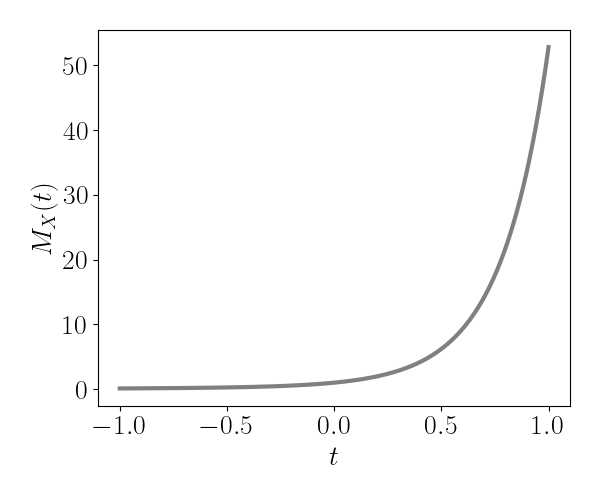
Intuitively, we can think of this distribution’s first moment as the slope of this curve at $t=0.$ The distribution’s second moment is given by this curve’s quadratic curvature at $t=0,$ and so on. More precisely, the moments are easily calculated from the derivatives of the MGF:

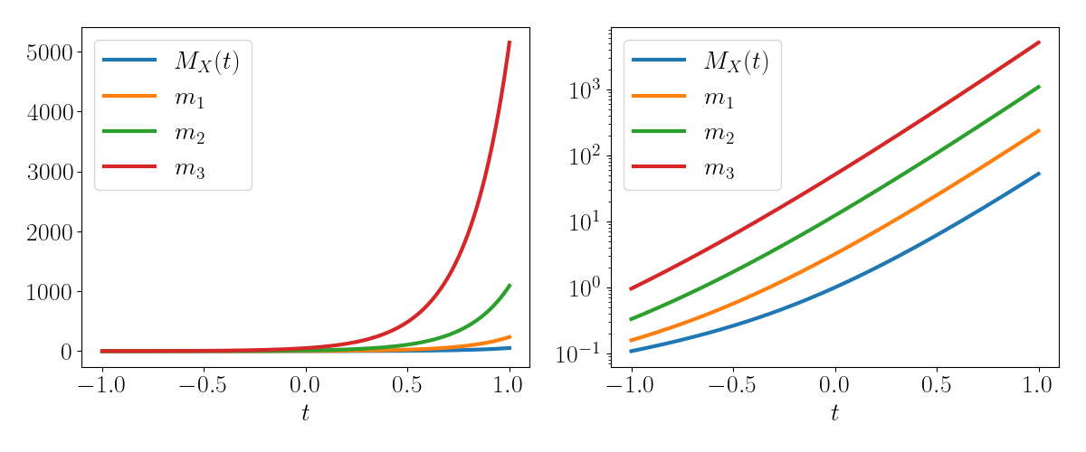
\begin{align} m_1 &= \sum\limits_{k=1}^K p_k x_k e^{t x_k} \\ m_2 &= \sum\limits_{k=1}^K p_k x_k^2 e^{t x_k} \\ m_3 &= \sum\limits_{k=1}^K p_k x_k^3 e^{t x_k} \\ &\quad\quad \vdots \end{align}

Recall that the moments are equal to the evaluation of these derivatives at $t=0.$ We visualize each of these derivatives below, where the left and right panels show the derivatives on the original and log scales, respectively:

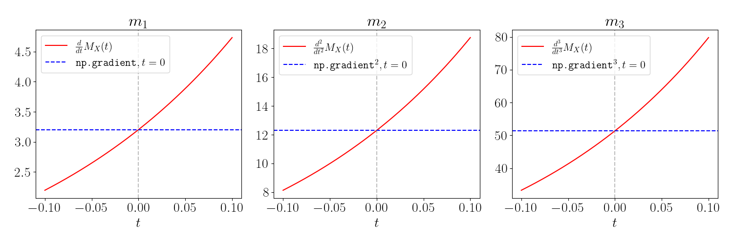
Let’s do some sanity checks to make sure that the empirical derivatives of the MGF are equal to those obtained by directly evaluating the moments. Below, we plot the first three $\color{red}{\text{derivatives of the MGF}}$ as $\color{red}{\text{red}}$ lines.

To compute an empirical estimate of each moment, we use the NumPy function $\texttt{np.gradient}$ applied to the MGF. To estimate the $n$th moment, we apply $\texttt{np.gradient}$ recursively $n$ times. In the plots below, the horizontal $\color{blue}{\text{blue}}$ lines show the $\color{blue}{\text{empirical estimate}}$ of each derivative at $t=0.$ For example, the code below computes an empirical estimate of the first derivative:

lims = [-1e0, 1e0]
ts = np.linspace(lims[0], lims[1], 401)
MXt = (np.exp(states * ts.reshape(-1, 1)) * ps).sum(1) # MGF
d1 = np.gradient(MXt, ts)                              # d/dt
m1 = d1[ts == 0]                                       # First moment at t=0

The vertical gray lines show $t=0,$ which is where we expect the blue and red lines to intersect (demonstrating agreement between the theoretical and empirical versions).

Example: Normal distribution

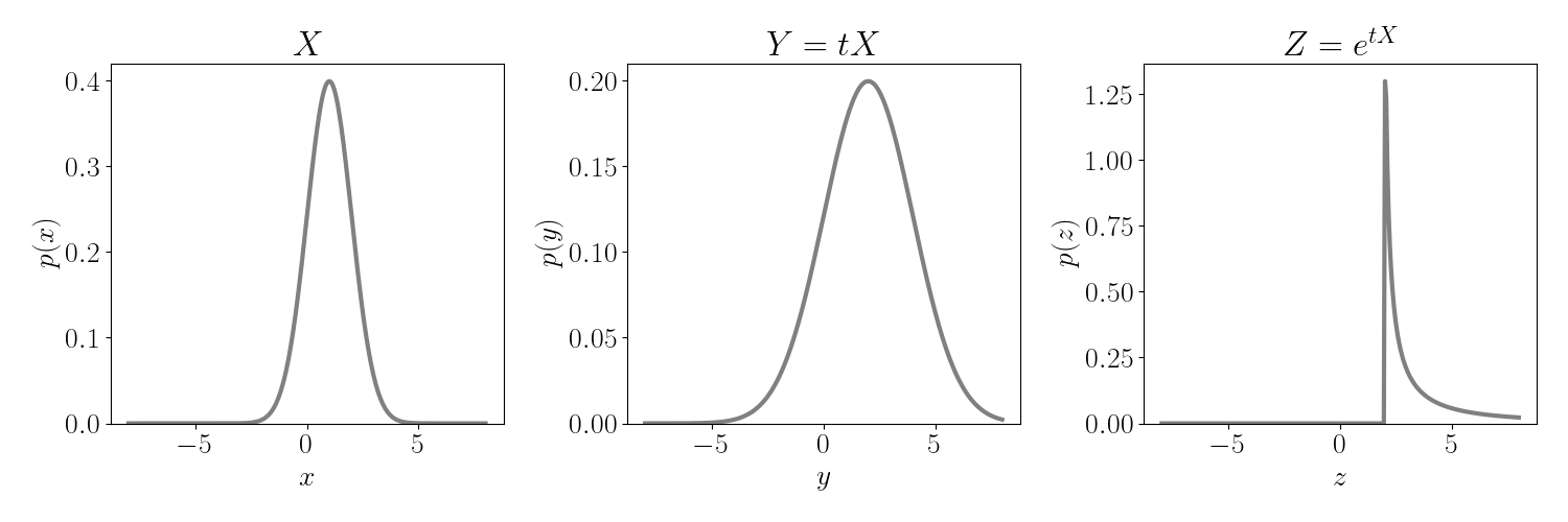
Consider a Gaussian random variable $X \sim N(\mu, \sigma^2).$ Recall that multiplying $X$ by a scalar $t$ results in another Gaussian random variable with scaled mean and variance:

Further, recall that exponentiating a Gaussian random variable results in a random variable with a log-normal distribution. That is,

These transformations of $X$ are shown visually below. Multiplication by $t$ scales the mean and variance, and exponentiating drastically changes the shape of the distribution.

In this case, the MGF corresponds with the mean of the log-normal random variable. By the distribution’s basic properties, the mean of the log-normal distribution is given by

We can then compute the Gaussian distribution’s moments from the derivatives of the MGF. For the first moment, we recover the distribution’s mean $\mu,$ which should intuitively make sense:

For the second moment, we differentiate again (using the product rule):

\begin{align} m_2 = &\Bigg[(\mu + \sigma^2 t)^2 \exp\left\{ t \mu + \frac12 t^2 \sigma^2 \right\} \\ &+ \sigma^2 \exp\left\{ t \mu + \frac12 t^2 \sigma^2 \right\}\Bigg]\bigg|_{t=0} = \mu^2 + \sigma^2. \end{align}

Note that when the mean is zero, $\mu = 0,$ we recover the variance $\sigma^2$ as the second central moment.

Calculation of the third moment follows a similar logic, again using the product rule:

\begin{align} m_3 = &\Bigg[(\mu + \sigma^2 t)^3 \exp\left\{ t \mu + \frac12 t^2 \sigma^2 \right\} \\ &+ 2 \sigma^2 (\mu + \sigma^2 t) \exp\left\{ t \mu + \frac12 t^2 \sigma^2 \right\} \\ &+ \sigma^2 (\mu + \sigma^2 t)\Bigg]\bigg|_{t=0} = \mu^3 + 3 \mu \sigma^2. \end{align}

Again, notice that when the mean is zero, $\mu = 0,$ we recover the fact that the third central moment is always zero, coinciding with the Gaussian distribution’s symmetry and lack of skew.

References

• Wikipedia page on moment-generating functions