Mixture of factor analyzers

\(\DeclareMathOperator*{\argmin}{arg\,min}\) \(\DeclareMathOperator*{\argmax}{arg\,max}\)

The mixture of factor analyzers model combines clustering and dimensionality reduction by allowing different regions of the data space to be modeled by different low-dimensional approximations. In this post, we introduce the two ingredients for the model — factor analysis and mixture models — and end by putting them together.

Factor analysis

Suppose we have a dataset of $n$ samples, $x_1, \dots, x_n$. Factor analysis assumes the following model for each data point $x_i \in \mathbb{R}^p$.

\begin{align} x_i &= W z_i + \epsilon_i \\ z_i &\sim \mathcal{N}(0, I_k) \\ \epsilon_i &\sim \mathcal{N}(0, \Psi) \end{align}

where $\Psi$ is a $p \times p$ diagonal covariance matrix. The latent variables $z_i$ are unobserved, lower-dimensional representations of the data points. The parameters in this case are the loading matrix $W$ and the noise covariance $\Psi$. We can’t directly find maximum likelihood solutions for these parameters due to the latent variables $z_i$, so we use expectation maximization (EM) instead. We give a brief review of EM for factor analysis below.

Recall that EM is an iterative algorithm, and suppose we’re currently on iteration $t+1$. In this case, our objective on iteration $t + 1$ is

\begin{equation} \max_{W, \Psi} Q = \max_{W, \Psi} \mathbb{E}_{z | x, W^t, \Psi^t} \left[ \sum\limits_{i=1}^n \log p(x_i, z_i | W, \Psi) \right] \tag{1} \label{eq:1} \end{equation}

where $W^t$ and $\Psi^t$ are the current parameter estimates. Expanding the log likelihood, we have

\begin{align} Q &= \sum\limits_{i=1}^n \mathbb{E}\left[ -\frac{p}{2} \log 2\pi - \frac{1}{2} \log |\Psi| - \frac12 (x_i - Wz_i)^\top \Psi^{-1} (x_i - Wz_i) \right] \\ &= -\frac{np}{2} \log 2\pi - \frac{n}{p} \log |\Psi| - \sum\limits_{i=1}^n \mathbb{E}\left[\frac12 (x_i - Wz_i)^\top \Psi^{-1} (x_i - Wz_i) \right]. \end{align}

Expanding the last term, we have

\begin{align} Q &= -\frac{np}{2} \log 2\pi - \frac{n}{p} \log |\Psi| \\ &- \frac12 \sum\limits_{i=1}^n x_i^\top \Psi^{-1} x_i + 2 \sum\limits_{i=1}^nx_i^\top \Psi^{-1} W \mathbb{E}[z_i] - \sum\limits_{i=1}^n \text{tr}\left(W^\top \Psi^{-1} W \mathbb{E}[z_i z_i^\top]\right). \end{align}

Taking the derivative with respect to $W$, we have

We can see that this will be zero when

\begin{equation} \widehat{W} = \left(\sum\limits_{i=1}^n x_i z_i^\top\right) \left( \sum\limits_{i=1}^n \mathbb{E}[z_i z_i]^\top] \right)^{-1}. \tag{2}\label{eq:2} \end{equation}

Now taking the derivative with respect to $\Psi^{-1}$, we have

Plugging in our estimate for $\widehat{W}$ in the last term, we have

\begin{align} \frac{\partial Q}{\partial \Psi^{-1}} &= \frac{n}{2} \Psi - \frac12 \sum\limits_{i=1}^n x_i x_i^\top + 2 \widehat{W} \sum\limits_{i=1}^n \mathbb{E}[z_i] x_i^\top - \sum\limits_{i=1}^n \left(\frac{\sum\limits_{i=1}^n x_i \mathbb{E}[z_i]^\top}{\left( \sum\limits_{i=1}^n \mathbb{E}[z_i z_i^\top] \right)^{-1}}\right) \mathbb{E}[z_i z_i^\top] \widehat{W}^\top \\ &= \frac{n}{2} \Psi - \frac12 \sum\limits_{i=1}^n x_i x_i^\top + 2 \widehat{W} \sum\limits_{i=1}^n \mathbb{E}[z_i] x_i^\top - \sum\limits_{i=1}^n x_i \mathbb{E}[z_i]^\top \widehat{W}^\top \\ &= \frac{n}{2} \Psi - \frac12 \sum\limits_{i=1}^n x_i x_i^\top + \widehat{W} \sum\limits_{i=1}^n \mathbb{E}[z_i] x_i^\top. \\ \end{align}

Solving for $\Psi$, this leaves us with

\begin{equation} \widehat{\Psi} = \frac{1}{n} \sum\limits_{i=1}^n x_i x_i^\top - \widehat{W} \sum\limits_{i=1}^n \mathbb{E}[z_i] x_i^\top. \tag{3}\label{eq:3} \end{equation}

The expectations of the latent variables $z_i$ and their outer products $z_i z_i^\top$ are given by

\begin{align} \mathbb{E}[z_i] &= \beta x_i \\ \mathbb{E}[z_i z_i^\top] &= I - \beta \Lambda + \beta x_i x_i^\top \beta^\top \end{align}

where $\beta = \Lambda^\top (\Psi + \Lambda \Lambda^top)^{-1}$.

At this point, we would proceed to the next iteration, using Equations \eqref{eq:2} and \eqref{eq:3} as our next parameter estimates, and optimize the objective function in Equation \eqref{eq:1}.

Mixture models

Next, we’ll briefly review Gaussian mixture models and how to use EM for estimation. Assume we have a dataset $\{x_i\}_{i=1}^n$, and we assume that each sample $x_i \in \mathbb{R}$ belongs to one of $K$ latent clusters. Furthermore, each of these clusters is modeled by its own Gaussian distribution. The generative model is as follows:

\begin{align} x_i | z_i = k &\sim \mathcal{N}(\mu_k, \sigma^2_k) \
p(z_i = k) &= \pi_k,~~~\sum\limits_{k=1}^K \pi_k = 1. \end{align}

Here, $z_i$ is a latent variable for $x_i$ indicating its mixture membership, and our goal is to estimate the mixture parameters $\theta_k = \{\mu_k, \sigma^2_k, \pi_k\}$. Since $z_i$ isn’t observed, we can’t simply maximize the likelihood of $x_i$ with respect to the parameters.

To circumvent this issue, EM instead forms an expected likelihood of the data, where the expectation is over the plausible values for $z_i$. Note that the posterior for $z_i$ is given by

Given a current estimate of the model parameters $\widetilde{\theta}_k$, we can then take an expectation of the likelihood with respect to this posterior:

We will then maximize this expected log likelihood with respect to $\theta_k$. First, let’s expand the expectation,

\begin{align} \mathbb{E}_{p(z_i = k | x_i, \widetilde{\theta}_k)}[\log p(x_i, z_i | \theta_k)] &= \sum\limits_{k=1}^K p(z_i = k | x_i, \widetilde{\theta}_k) \log p(x_i, z_i | \theta_k) \\ &= \sum\limits_{k=1}^K \frac{p(x_i | z_i = k, \widetilde{\theta}_k) \pi_k}{\sum\limits_{k^\prime=1}^K p(x_i | z_i = k^\prime, \widetilde{\theta}_{k^\prime}) \pi_{k^\prime}} \log p(x_i, z_i | \theta_k) \end{align}

where we have plugged in the posterior for $z_i$. To simplify notation, let’s define

Then our expectation becomes

Writing out the expected likelihood for the entire dataset (not just the $i$th point), we have

We can now maximize with respect to $\theta_k$. Let’s start by optimizing $\mu_k$, and let’s write out the expected log likelihood in more detail and drop terms that don’t depend on $\mu_k$.

\begin{align} \mathcal{L}(\theta_k) &= \sum\limits_{i=1}^n \sum\limits_{k=1}^K \gamma_{ik} \left(\log \pi_k - \log 2\pi \sigma^2_k - \frac{1}{2\sigma^2_k}(x_i - \mu_k)^2\right) \\ &= (\log \pi_k - \log 2\pi \sigma^2_k) \sum\limits_{i=1}^n \gamma_{ik} - \frac{1}{2\sigma^2_k} \sum\limits_{i=1}^n (x_i^2 - 2x_i \mu_k + \mu_k^2) \\ &= \underbrace{(\log \pi_k - \log 2\pi \sigma^2_k) \sum\limits_{i=1}^n \gamma_{ik} - \frac{1}{2\sigma^2_k} \sum\limits_{i=1}^n \gamma_{ik} x_i^2}_{C} - \frac{1}{2\sigma^2_k} \sum\limits_{i=1}^n \gamma_{ik} (-2x_i \mu_k + \mu_k^2). \\ \end{align}

Here, $C$ is constant with respect to $\mu_k$. Taking the derivative wrt $\mu_k$, we have

Setting this to zero, we find that the optimal $\mu_k$ is given by

Thus, $\widehat{\mu}_k$ is just a weighted average of the data, where the weights are the posterior expectations of each sample’s mixture membership. Plugging this back into $\mathcal{L_k}$ and optimizing $\sigma^2_k$, we have

\begin{align} \mathcal{L}(\theta_k) &= \underbrace{(\log \pi_k - \log 2\pi) \sum\limits_{i=1}^n \gamma_{ik}}_{C} - \log \sigma^2_k \sum\limits_{i=1}^n \gamma_{ik} - \frac12 (\sigma^{2}_k)^{-1} \sum\limits_{i=1}^n \gamma_{ik} (x_i - \widehat{\mu}_k)^2. \\ \end{align}

Taking the derivative wrt $\sigma^2_k$, we have

\begin{align} \frac{\partial \mathcal{L}}{\partial \sigma^2_k} &= \frac{1}{\sigma^2_k} \sum\limits_{i=1}^n \gamma_{ik} + (\sigma^{2}_k)^{-2} \sum\limits_{i=1}^n \gamma_{ik} (x_i - \widehat{\mu}_k)^2 \\ &= \frac{1}{\sigma^2_k} \left( \sum\limits_{i=1}^n \gamma_{ik} - \frac{1}{\sigma^2_k} \sum\limits_{i=1}^n \gamma_{ik} (x_i - \widehat{\mu}_k)^2 \right). \end{align}

Setting this to zero, we find that the optimal $\sigma^2_k$ is given by

Finally, optimizing $\pi_k$, we have

We also must enforce the constraint that $\sum\limits_{k^\prime = 1}^K \pi_{k^\prime} = 1$. We can do this using Lagrange multipliers. The objective function is

The gradient will be

Setting these to zero, we see that the optimal mixing proportions are given by

Mixtures of factor analyzers

Factor analysis assumes one linear model can model the entire data space. However, a more flexible approach is to allow for different regions of the data space to be modeled differently. For this purpose, Ghahramani and Hinton proposed mixtures of factor analyzers. This model is essentially a hybrid of a linear dimensionality reduction method (factor analysis) and a clustering method (Gaussian mixture model).

To start, let’s define the model. We assume there are $K$ separate factor analysis models, each of which with its own parameters. Let $\omega_{ik}$ be an indicator variable such that

Then, conditioned on $\omega_{ik}$, the model is

\begin{align} x_i | \{\omega_{ik}\} &= \prod\limits_{k=1}^K \left(\Lambda_k z_{ik} + \mu_k + \epsilon_i\right)^{\omega_{ik}} \\ z_{ik} &\sim \mathcal{N}(0, I_d) \\ \epsilon_i &\sim \mathcal{N}(0, \Psi). \end{align}

The marginal distribution of $x_i$ is

Estimation for this model proceeds similarly to factor anlaysis and mixture models using EM. On each iteration, we first compute the expectation of the complete data log likelihood with respect to the posterior over $z$, and then we maximize this likelihood with respect to the model parameters. The main thing that changes from factor analysis is that now we have $K$ sets of parameters to estimate.

In factor analysis, we could assume that the data was mean-centered without loss of generality. In this case, we have multiple components, so we must have a mean $\mu_k$ for each component as well. To simplify notation and computation, we’ll assume that the mean is appended to $\Lambda_k$ such that

We also add an element of one to the latent variables $z$,

Then, the mean contributes naturally through the matrix product $\Lambda_k z_i$.

To compute the EM updates, let’s first write out the complete data log likelihood.

\begin{align} &p(x, z | \Lambda, \Psi) = \log \prod\limits_{i=1}^n \prod\limits_{k=1}^K \left[p(x_i, z_{ik} | \Lambda_k, \Psi)\right]^{\omega_{ik}} \\ &= \sum\limits_{i=1}^n \sum\limits_{k=1}^K \omega_{ik} \left[ \log p(x_i, z_{ik} | \Lambda_k, \Psi)\right] \\ &= \sum\limits_{i=1}^n \sum\limits_{k=1}^K \omega_{ik} \left( -\frac{D}{2} \log 2\pi - \frac12 \log |\Psi| - \frac12 (x_i - \Lambda_k z_{ik})^\top \Psi^{-1} (x_i - \Lambda z_{ik}) \right) \\ &= -\frac{nD}{2} - \frac{n}{2} \log |\Psi| - \frac12 \sum\limits_{i=1}^n \sum\limits_{k=1}^K \omega_{ik} (x_i - \Lambda_k z_{ik})^\top \Psi^{-1} (x_i - \Lambda z_{ik}) \\ &= C - \frac{n}{2} \log |\Psi| - \sum\limits_{i=1}^n \sum\limits_{k=1}^K \left(\frac12 \omega_{ik} x_i^\top \Psi^{-1} x_i - \omega_{ik} x_i^\top \Lambda_k z_{ik} + \frac12 \omega_{ik} z_{ik}^\top \Lambda_k^\top \Psi^{-1} \Lambda_k z_{ik}\right) \\ &= C - \frac{n}{2} \log |\Psi| - \sum\limits_{i=1}^n \sum\limits_{k=1}^K \left(\frac12 \omega_{ik} \text{tr}(\Psi^{-1} x_i x_i^\top) - \omega_{ik} x_i^\top \Lambda_k z_{ik} + \frac12 \omega_{ik} \text{tr}(\Lambda_k^\top \Psi^{-1} \Lambda_k z_{ik} z_{ik}^\top) \right). \\ \end{align}

Taking the expectation with respect to the posterior, we have

\begin{align} &\mathbb{E}[p(x | z, \Lambda, \Psi)] \\ =& C - \frac{n}{2} \log |\Psi| - \sum\limits_{i=1}^n \sum\limits_{k=1}^K \left(\frac12 \mathbb{E}[\omega_{ik}] \text{tr}(\Psi^{-1} x_i x_i^\top) - \mathbb{E}[\omega_{ik}] x_i^\top \Lambda_k \mathbb{E}[z_{ik}] + \frac12 \mathbb{E}[\omega_{ik}] \text{tr}(\Lambda_k^\top \Psi^{-1} \Lambda_k \mathbb{E}[z_{ik} z_{ik}^\top]) \right). \end{align}

To compute the expectations, notice that

Let’s compute these.

\begin{align} \mathbb{E}[\omega_{ik}] &= \sum\limits_{k=1}^K \omega_{ik} p(\omega_{ik} | x_i, \Lambda_k, \Psi) \\ &= \sum\limits_{k=1}^K \frac{p(x_i | \omega_{ik}, \Lambda_k, \Psi) p(\omega_{ik})}{\sum\limits_{k^\prime=1}^K p(\omega_{ik^\prime}, x_i, \Lambda_{k^\prime}, \Psi)} \\ &= \sum\limits_{k=1}^K \frac{\pi_k \mathcal{N}(x_i | 0, \Lambda_k \Lambda_k^\top + \Psi)}{\sum\limits_{k^\prime=1}^K \pi_{k^\prime} \mathcal{N}(x_i | 0, \Lambda_{k^\prime} \Lambda_{k^\prime}^\top + \Psi)}. \end{align}

We can see that this expectation closely resembles that of the Gaussian mixture model, where the expectation of each cluster membership is the (normalized) likelihood of the data under that cluster’s parameters.

The expectations of $z_i$ are identical to those for factor analysis, but we use the component-specific parameterss (including the mean offset):

\begin{align} \mathbb{E}[z_i | \omega_{ik}] &= \mathbb{E}[\omega_{ik}] \beta_k (x_i - \mu_k) \\ \mathbb{E}[z_i z_i^\top | \omega_{ik}] &= \left( I - \beta_k \Lambda_k + \beta_k (x_i - \mu_k) (x_i - \mu_k)^\top \beta_k^\top \right) \end{align}

where again $\beta_k = \Lambda_k^\top (\Psi + \Lambda \Lambda^\top)^{-1}$.

Plugging these into the objective function, taking derivatives with respect to $\Lambda_k$ and $\Psi$ (much of which is very similar computation to that for factor analysis), we find the following parameter updates.

\begin{align} \widehat{\Lambda}_k &= \left( \sum\limits_{i=1}^n \mathbb{E}[\omega_{ik}] x_i \mathbb{E}[z_i | x_i, \omega_{ik}]^\top \right) \left( \sum\limits_{i=1}^n \mathbb{E}[\omega_{ik}] \mathbb{E}[z_i z_i^\top | x_i, \omega_{ik}]^\top \right)^{-1} \\ \widehat{\Psi} &= \frac1n \text{diag}\left\{ \sum\limits_{i=1}^n \sum\limits_{k=1}^K \mathbb{E}[\omega_{ik}] \left( x_i - \widehat{\Lambda}_k \mathbb{E}[z_i | \omega_{ik}] \right) x_i^\top \right\}. \end{align}

Let’s now see how this works in practice.

Experiment

Let’s consider a simple example. Suppose we have the two-dimensional dataset depicted below, where the points of each color are generated from one of three unique Gaussians.

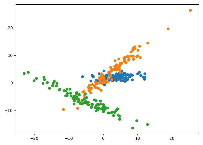
As we can see, each cluster of data has one major axis of variation. We can fit the mixture of factor analyzers model to identify these unique clusters. Specifically, we set the number of components to be $K=3$, and we run EM to estimate $\{\Lambda_k\}_{k=1}^K$ and $\Psi$. Here, we use just one latent dimension.

Below is an animation showing the iterative steps taken by EM in this case. Each black line represents the line represented by one $\Lambda_k$. The midpoint of each line represents the component mean.

Furthermore, we can visualize the fractional membership of each point in each cluster. Below, we color the points by $\mathbb{E}[w_{ik}]$ for each value of $k$.

As the mixtures settle into their optima, each mixture component takes more responsbility for its respective points, as shown by the brighter colors within each cluster in the animations above.

Conclusion

Using mixtures of factor analyzers can make for very expressive models. A simple factor analysis model is a drast oversimplification in most real-world data. In other words, the data typically isn’t distributed as a big multivariate Gaussian with a low-rank covariance matrix. However, using mixtures of Gaussians lets us model different regions of the data with different covariance matrices, which is quite flexible.

References

• Ghahramani, Zoubin, and Geoffrey E. Hinton. The EM algorithm for mixtures of factor analyzers. Vol. 60. Technical Report CRG-TR-96-1, University of Toronto, 1996.
• Greg Gundersen’s blog post on factor analysis.
• Prof. Matthew Stephen’s post on EM for Gaussian mixture models.

Code

import numpy as np
import matplotlib.pyplot as plt
import seaborn as sns
from scipy.stats import multivariate_normal as mvn
import os
from os.path import join as pjoin

np.random.seed(13)

K = 3
n = 100
D = 2
d = 1
X = np.zeros((n*K, D))

# Loadings
Lambda = np.random.normal(scale=5, size=(K, D, d+1))

# Noise covariance
Psi = np.diag(np.ones(D))

# Latent variables
z = np.random.normal(size=(d, n*K))
z = np.concatenate([z, np.ones((1, n*K))])

mvn_gen = mvn(mean=np.zeros(D), cov=Psi)

for k in range(K):

	# Generate data
	k_idx = np.arange(k * n, (k + 1) * n)
	curr_data = (Lambda[k] @ z[:, k_idx]).T + mvn_gen.rvs(n)
	X[k_idx] = curr_data


X = X.T

## Fit EM

Lambda_est = np.random.normal(scale=10, size=(K, D, d+1))
Psi_est = np.diag(np.ones(D))
pi = np.ones(K) / K
h = np.ones((K, n*K))
n_iters = 40

for ii in range(n_iters):

	# Compute h
	for k in range(K):

		L = Lambda_est[k][:, :d]
		mu = Lambda_est[k][:, d:]
		
		h[k, :] = pi[k] * mvn(mean=mu.squeeze(), cov=L @ L.T + Psi_est).pdf(X.T)

	h = h / np.sum(h, axis=0)

	Psi_new = np.zeros((D, D))
	for k in range(K):

		# Compute beta
		L = Lambda_est[k][:, :d]
		mu = Lambda_est[k][:, d:]
		X_centered = X - mu
		beta = L.T @ np.linalg.inv(Psi_est + L @ L.T)

		# Compute expectations
		Ez = beta @ X_centered
		Ez = np.concatenate([Ez, np.ones((1, n*K))])

		EzzT = np.zeros((d+1, d+1))
		EzzT[:d, :d] = np.sum(h[k]) * (np.eye(d) - beta @ L) + beta @ (h[k] * X_centered) @ X_centered.T @ beta.T

		EzzT_offdiag_term = np.sum(h[k] * Ez[:d, :], axis=1)
		EzzT[:d, d:] = EzzT_offdiag_term
		EzzT[d:, :d] = EzzT_offdiag_term.T
		EzzT[d:, d:] = np.sum(h[k])
		
		# Update parameters
		Lambda_est[k] = (h[k] * X) @ Ez.T @ np.linalg.inv(EzzT)
		Psi_new += np.diag(np.diag((X - Lambda_est[k] @ Ez) @ ((h[k] * X).T)))

	Psi_est = Psi_new / (n * K)

	# Update pi
	pi = np.mean(h, axis=1)