Andy Jones
Equivalence of mixed models and hierarchical models
Mixed models are effectively a special case of hierarchical models. In this post, I try to draw some connections between these jargon-filled modeling approaches.
Introduction
Consider $n$ samples $y_1, \dots, y_n$, each of which belongs to one of $J$ groups. We use the notation $y_{ij}$ to refer to sample $i$ which belongs to group $j$.
We’re often interested in describing the data at multiple levels: both as one homogeneous group and in terms of group-specific characteristics. Several modeling approaches allow for this. However, there is quite a bit of nomenclature that ultimately refers to the same or very similar models. Here, I review two of these types of models that have different names but are ultimately the same in many cases: mixed models and hierarchical models.
Linear mixed models
Linear mixed models consist of both “fixed” and “random” effects (hence the name “mixed effects”). Generically, these models can be written in the form
\[Y = X \alpha + D \beta + \epsilon\]where $X$ is an $n\times p$ matrix of covariates, $\alpha \in \mathbb{R}^p$ is a vector of fixed effects, $D \in \{0, 1\}^{n\times J}$ design matrix indicating each samples group membership, and $\beta \in \mathbb{R}^J$ is a vector of random effects. For a single sample, we can write
\[y_{ij} = x_i \alpha + d_i \beta_j + \epsilon\]where $x_i$ and $d_i$ are the $i$th rows of $X$ and $D$, and $\beta_j$ is the $j$th element of $\beta$.
The coefficient vector $\beta$ is random, and thus we must make an assumption about its distribution. We typically assume
\[\beta \sim \mathcal{N}(0, \Sigma)\]where $\Sigma$ is the covariance of the random effects coefficients. Intuitively, we can think of $\Sigma$ as encoding the relationships between groups $j=1, \dots, J$. For example, if the “groups” are different genetic strains of mice, $\Sigma$ will encode any known relatedness between the strains.
Hierarchical models
The combination of fixed and random effects will feel unnatural to a Bayesian — in a fully Bayesian framework, we would think of all of these quantities as random. So-called hierarchical models have more of a Bayesian flavor.
A hierarchical model analogous to the LMM above can be written as
\begin{align} y_{ij} &\sim \mathcal{N}(\beta_j, \tau^2 I) ~~~ \text{for } j=1,\dots,J \\ (\beta_1, \dots, \beta_J)^\top &\sim \mathcal{N}(x_i \alpha, \Sigma) \\ \alpha &\sim \pi \end{align}
where $\pi$ is the prior for $\alpha$ (assume $\tau^2$ is known for now). Here, we have parameterized the mean of the coefficients $\{\beta_j\}$ with a linear function of the covariates $X$.
Notice that we can translate the mixed effects language into this framework. In the hierarchical model formulation, the “fixed effects” (which are shared across all groups) are given by the shared parameterization of the mean through $\alpha$. The random effects (which are group-specific) are implied by the group-specific means $\{\beta_j\}$. Notice that we no longer need the design matrix $D$ in this notation.
Using different notation, we can write this model as
\begin{align} y_i &= X\alpha + D\beta + \epsilon \\ (\beta_1, \dots, \beta_J)^\top &\sim \mathcal{N}(0, \Sigma) \\ \alpha &\sim \pi \\ \epsilon &\sim \mathcal{N}(0, \tau^2I) \end{align}
In this case $D$ is again the $n\times J$ design matrix indicating the group membership of each sample.
This is getting closer to looking like a linear mixed model, but we’re not quite there. The one remaining difference is the prior for $\alpha$. Recall that in mixed models, there was no randomness in $\alpha$, so it doesn’t make sense to place an informative prior on it.
To fully recover the mixed model setting, we can place a uniform, non-informative, improper prior on alpha:
\[p(\alpha) \propto 1.\]Then, we can effectively think of $\alpha$ as being non-random (although this isn’t entirely true), and we recover the mixed model setup.
Common assumption
A common assumption is that $\beta_1, \dots, \beta_J$ are independent:
\[(\beta_1, \dots, \beta_J)^\top \sim \mathcal{N}(0, \sigma^2 I).\]In this case, we assume each $\beta_j$ has mean $0$ and shared variance $\sigma^2$. This is similar to including a ridge ($L_2$) penalty to a classical regression setting.
Simple example
Consider the case where we have $J=4$ groups, and we’d like to model the group-specific mean while accounting for a one-dimensional covariate $X$. In other words, our model is
\begin{align} y_{ij} &\sim \mathcal{N}(x_i \alpha + \beta_j, \tau^2) \\ \beta_j &\sim \mathcal{N}(0, \sigma^2). \end{align}
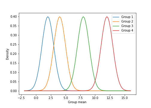
Suppose we observe some data with group means
\[\begin{bmatrix} \beta_1 \\ \beta_2 \\ \beta_3 \\ \beta_4 \end{bmatrix} = \begin{bmatrix} 2 \\ 4 \\ 8 \\ 12 \end{bmatrix}.\]The outcome variable $Y$ then has a group-specific density that looks like this:
However, suppose the covariate $X$ is highly inversely correlated with the group mean ($x_{ij} \approx -\beta_j$). In this case, we might observe data that looks like this:
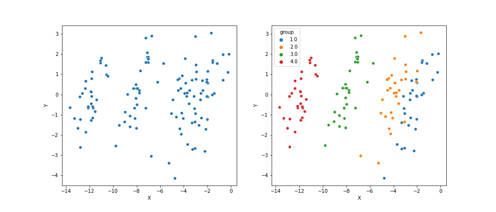
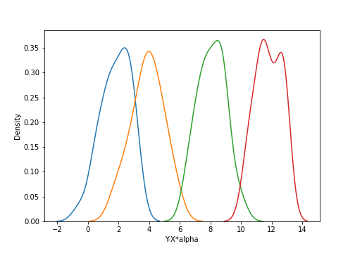
In the left plot, it appears that there’s no relationship between $X$ and $Y$. However, the right plot makes it clear that there’s group-specific structure. If we correct for the covariate $X$ and instead look at the density of $Y-X\alpha$, we have the following:
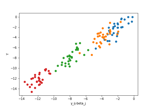
Conversely, if we correct for the group-specific means, and look at the covariate $X$ versus the residuals $y_{ij} - \beta_j$, we have
Code
The code for the simple demonstration above is below.
import numpy as np
import matplotlib.pyplot as plt
import seaborn as sns
import pandas as pd
from scipy.stats import norm

group_means = np.array([2, 4, 8, 12])
group_var = 1

## Plot group-specific densities
xs = np.linspace(np.min(group_means)-4, np.max(group_means)+4, 100)
density_list = []
plt.figure(figsize=(7, 5))
for ii, gm in enumerate(group_means):
    ds = norm.pdf(xs, gm)
    plt.plot(xs, ds, label="Group {}".format(ii+1))
plt.legend()
plt.xlabel("Group mean")
plt.ylabel("Density")
plt.show()

## Generate data
nj = 30
D = np.zeros((nj*len(group_means), len(group_means)))
D_num = np.zeros(nj*len(group_means))
X = np.zeros(nj*len(group_means))
Y = np.zeros(nj*len(group_means))
alpha = 1
for ii, gm in enumerate(group_means):
    D[ii*nj:(ii+1)*nj] = 1
    D_num[ii*nj:(ii+1)*nj] = ii + 1
    X[ii*nj:(ii+1)*nj] = -group_means[ii] + np.random.normal(size=nj)
    Y[ii*nj:(ii+1)*nj] = X[ii*nj:(ii+1)*nj] * alpha + group_means[ii] + np.random.normal(size=nj)

## Scatter plot of data
data = pd.DataFrame({'X': X, 'Y': Y, 'group': D_num.astype(str)})
plt.figure(figsize=(14, 6))
plt.subplot(121)
sns.scatterplot(data=data, x="X", y="Y") #, hue="group")
plt.subplot(122)
sns.scatterplot(data=data, x="X", y="Y", hue="group")
plt.savefig("./out/XY_lmm.png")
plt.show()

## Density of covariate-corrected data
Y_corrected = data.Y - data.X * alpha
plt.figure(figsize=(7, 5))
for ii, gm in enumerate(group_means):
    sns.distplot(Y_corrected[ii*nj:(ii+1)*nj], hist=False)
# plt.legend()
plt.xlabel("Y-X*alpha")
plt.ylabel("Density")
plt.savefig("./out/group_densities_corrected_lmm.png")
plt.show()

## Scatter of group-corrected data
plt.figure(figsize=(7, 5))
for ii, gm in enumerate(group_means):
    plt.scatter(X[ii*nj:(ii+1)*nj], data.Y[ii*nj:(ii+1)*nj] - gm)
# plt.legend()
plt.xlabel("y_ij-beta_j")
plt.ylabel("Y")
plt.savefig("./out/XY_lmm_corrected.png")
plt.show()
References
- Gelman, Andrew, et al. Bayesian data analysis. CRC press, 2013.
- Zhou, Xiang, and Matthew Stephens. “Genome-wide efficient mixed-model analysis for association studies.” Nature genetics 44.7 (2012): 821.
- Post from UCLA on linear mixed models.