Andy Jones
Common matrix decompositions
Matrix decomposition methods factor a matrix $A$ into a product of two other matrices, $A = BC$. In this post, we review some of the most common matrix decompositions, and why they’re useful.
Introduction
Matrix decompositions are very general tools in linear algebra. They’re useful for a variety of applications, like solving linear systems of equations, inverting matrices, and implementing statistical methods.
QR decomposition
The QR decomposition can decompose any square matrix $A \in \mathbb{R}^{n\times n}$ as
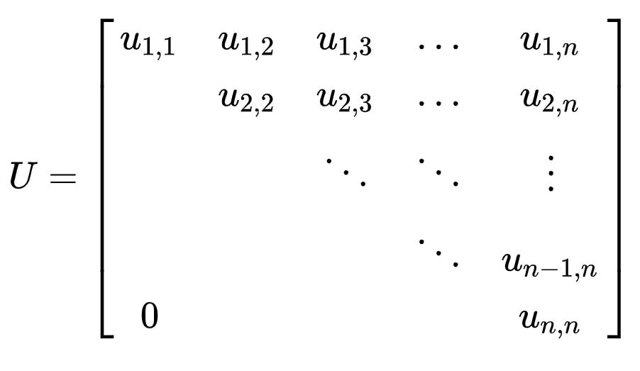
\[A = QR\]where $Q$ is an $n \times n$ orthogonal matrix, and $R$ is an upper triangular matrix. As a refresher recall that a matrix $Q$ is orthogonal if $Q^\top Q = I$ and $QQ^\top = I$, and a matrix is upper triangular if all of its entries below the main diagonal are zero. That is, it looks something like:
The most common method for computing the QR decomposition is via the Gram-Schmidt process. The Gram-Schmidt process provides a way of finding an orthonormal basis for a full-rank matrix. Informally, the process proceeds in two steps for a column $i$ of the matrix $A$ (the one to be decomposed):
- Subtract the projection of the column $a_i$ onto the orthonormal vectors found for columns $1, \dots, i - 1$. Call this vector $u_i$.
- Normalize $u_i$ to have length $1$.
More formally, let the projection of a vector $a$ onto another vector $u$ be defined as
\[\text{proj}_u a = \frac{\langle u, a \rangle}{\langle u, u \rangle} u.\]Now to find an orthonormal basis for $A$, we go column by column and orthogonalize each of them. To begin, we take the first column of $A$, $a_1$ to be the first basis vector $u_1$. Then, we normalize this to get $q_1 = \frac{u_1}{||u_1||}$.
Next, to orthogonalize the second column of $A$, $a_2$, we subtract out its projection onto $q_1$ and normalize. Specifically, we take
\[u_2 = a_2 - \text{proj}_{u_1} a_2\] \[q_2 = \frac{u_2}{||u_2||}.\]More generally, for column $a_i$, we have
\[u_i = a_i - \sum\limits_{j = 1}^{i-1}\text{proj}_{u_j} a_i\] \[q_i = \frac{u_i}{||u_i||}.\]We can then take $Q$ to be the concatenation of $q_1, \dots, q_n$:
\[Q = [\mathbf{q_1} \; \mathbf{q_2} \; \cdots \; \mathbf{q_n}].\]Now to find $R$, we must find a way to express the columns $a_1, \dots, a_n$ in terms of our new orthonormal basis vectors $q_1, \dots q_n$. Recall that in general, a vector $v$ can be expressed in terms of an orthonormal basis $e_1, \dots, e_k$ as
\[\sum\limits_{i = 1}^k \langle e_i, v \rangle e_i.\]For each basis vector, we can think of $e_i$ as the direction of the vector, and the inner product $\langle e_i, v \rangle$ as determining the length of the vector.
Now, notice that we constructed $Q$ so that the $i$th column only depends on the previous $i-1$ columns. Therefore, the sum above in our case simplifies to
\[a_i = \sum\limits_{j = 1}^{i} \langle q_j, a_i \rangle q_j.\]Writing this out more fully, we have
\[a_1 = \langle q_1, a_1 \rangle q_1\] \[a_2 = \langle q_1, a_2 \rangle q_1 + \langle q_2, a_2 \rangle q_2\] \[a_3 = \langle q_1, a_3 \rangle q_1 + \langle q_2, a_3 \rangle q_2 + \langle q_3, a_3 \rangle q_3\] \[\dots\]We can see a triangular matrix starting to form. Specifically, the matrix $R$ will be
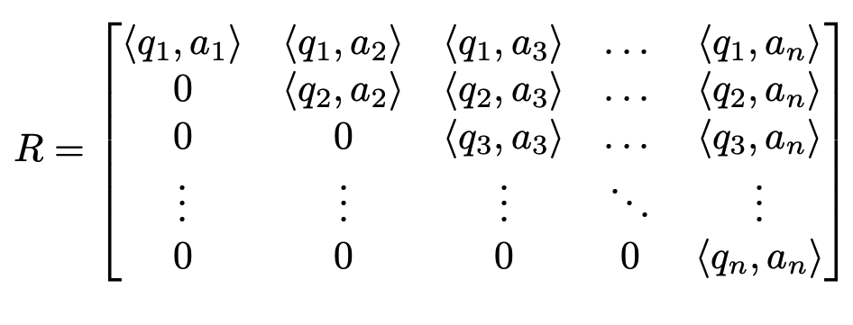
That finishes the QR decomposition. Thus, we can see the decomposition falls out almost naturally from orthonormalizing the matrix $A$.
Why is it useful?
The QR decomposition is widely used for solving linear systems of equations and computing matrix inverses. In particular, it’s useful for avoiding numerical instability in computing matrix inverses directly.
Consider, for example, the least-squares coefficient estimator:
\[\hat{\beta} = (X^\top X)^{-1} X^\top Y.\]Computing the inverse $(X^\top X)^{-1}$ can lead to under- or over-flow issues when $X^\top X$ has values that vary widely in magnitude.
Using the QR decomposition, we can avoid directly instantiating $X^\top X$, and instead use a more numerically stable instance of the problem.
Recall that to minimize the sum of squared errors, we must solve the problem
\[\min_\beta (Y - X\beta)^\top (Y - X\beta).\]Taking a derivative w.r.t. $\beta$, this means we must solve
\[-X^\top Y + X^\top X \beta = 0 \implies X^\top X \beta = X^\top Y.\]Performing a QR decomposition on $X$ and substituting $X = QR$, we have
\begin{align} X^\top X \beta &= X^\top Y \\ (QR)^\top QR \beta &= (QR)^\top Y \\ R^\top \underbrace{Q^\top Q}_{I_n} R \beta &= R^\top Q^\top Y \\ R^\top R \beta &= R^\top Q^\top Y \\ R \beta &= Q^\top Y && \text{(left multiply by $R^\top$)}. \\ \end{align}
Then, this system of equations is more stable and can be solved with functions that take advantage of the upper triangular structure of $R$ (e.g., “backsolve” in R).
Other notes about the QR decomposition
While the Gram-Schmidt process is intuitive and can be easily implemented as an algorithm, it can be numerically unstable. The repeated use of projections can cause numerical error.
LU decomposition
The LU decomposition is another type of factorization that’s useful for solving systems of linear equations. It decomposes a matrix $A$ into the product of a lower-triangular matrix and an upper-triangular matrix, $A = LU$. For a $3 \times 3$ matrix, this looks like (image from Wikipedia):
The LU decomposition is essentially a form of Gaussian elimination that, instead of computing row operations by hand, uses matrices. Recall that Gaussian elimination puts a matrix into row echelon form by adding rows, swapping rows, and multiplying rows by scalar values (and combinations of those operations). We can think of $U$ as the version of $A$ that has been reduced to row echelon form, and we can think of $L$ as representing the series of operations to achieve that form.
Let’s start with a simple example of reducing a matrix to row echelon form. Consider the following matrix.
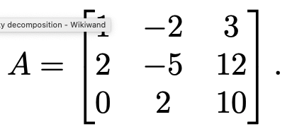
The first step of Guassian elimination would proceed to add $-2$ times Row 1 to Row 2, resulting in the matrix
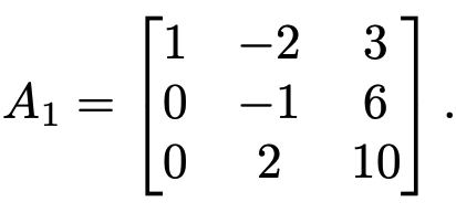
Notice that this operation could have also been performed by left-multiplying $A$ by
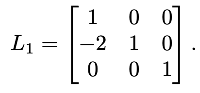
In other words, $L_1 A = A_1 \implies A = L_1^{-1} A_1$.
If we carry out all of the steps for Guassian elimination, we’ll end up with a set of matrices $L_1, \dots, L_n$ that perform the required operations. In addition, it will be true that
\[A = \underbrace{L_1^{-1} L_2^{-1} \dots L_n^{-1}}_L \underbrace{A_{n-1}}_U\]where $L$ is a matrix representing the steps of Gaussian elimination (with zeros above the main diagonal), and $U$ is a matrix representing the matrix is reduced echelon form (with zeros below the main diagonal). Thus, we have an LU decomposition.
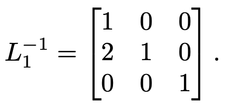
Now it remains to be seen whether we can find a nicer expression for the series of inverse matrices $L_1^{-1} L_2^{-1} \dots L_n^{-1}$. Notice, for example, that for $L_1$, the inverse can be found by negating the off-diagonal elements (just the $-2$ in this case):
This will be true for all of the $L_1, \dots, L_n$. After multiplying these matrices through ($L_1^{-1} L_2^{-1} \dots L_n^{-1}$), we’ll end up with a lower-triangular matrix $L$ each of whose columns represents the negation of its respective Gaussian elimination step. This is known as the Doolittle algorithm for computing an LU decomposition.
Cholesky decomposition
The Cholesky decomposition is very similar in spirit to the LU decomposition. It decomposes a positive (semi-)definite matrix $A$ into a product between a lower-triangular matrix $L$ and its conjugate transpose:
\[A = LL^*.\]For the purposes of this post, we’ll assume $A$ is positive definite, symmetric, and real, $A \in \mathbb{R}^{n \times n}$. Then the decomposition is
\[A = LL^\top.\]This type of decomposition is especially useful when dealing with covariance matrices.
The most straightforward algorithm for computing a Cholesky decomposition – the Cholesky algorithm – again performs Guassian elimination at its core.
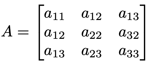
Consider a $3 \times 3$ positive definite matrix $A$:
We want to find a decomposition that looks like
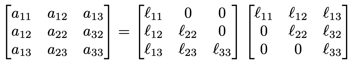
In some sense, we can think of the decomposition of $A = LL^\top$ as finding the “square root” of $A$. The Cholesky algorithm starts at the top-left element $a_{11}$, solves for this element, and iteratively solves for elements down and to the right.
To find $\ell_{11}$, we have the simple computation
\[a_{11} = \ell_{11}\ell_{11} \implies \ell_{11} = \sqrt{a_{11}}.\]This allows us to find the elements $\ell_{12}$ and $\ell_{13}$ (the first column of $L$ and the first row of $L^\top$.
\begin{align} &a_{12} = \ell_{11} \ell{12} = \sqrt{a_{11}} \ell_{12} \\ \implies& \ell_{12} = \frac{1}{\sqrt{a_{11}}} a_{12}. \end{align}
Similarly, we have $\ell_{13} = \frac{1}{\sqrt{a_{11}}} a_{13}$.
So far, we have computed $L$ as
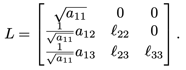
The remaining unknown elements are $\ell_{22}$, $\ell_{23}$, and $\ell_{33}$. If $A$ were larger than $3 \times 3$, we could think of these as three submatrices $B$, $C$, and $D$.
To compute $\ell_{22}$, we do another bit of simple algebra:
\begin{align} &a_{22} = \frac{1}{\sqrt{a_{11}}} a_{12} \frac{1}{\sqrt{a_{11}}} a_{12} + \ell_{22}^2 \\ \implies & \ell_{22} = \sqrt{a_{22} - \frac{1}{\sqrt{a_{11}}} a_{12} \frac{1}{\sqrt{a_{11}}} a_{12}}. \end{align}
This process repeats iteratively until all elements are found. Similar to the LU decomposition, these steps can be represented as a series of matrix multiplications, which make for safer bookkeeping (see the Cholesky algorithm section of this Wikipedia page.
Applications of the Cholesky decomposition include solving systems of linear equations and generating random variables with a particular covariance matrix (e.g., for Gaussian processes, or generally in Monte Carlo settings). For a vector $\mathbf{v}$ of uncorrelated random variables, we can induce the covariance structure specified by some matrix $A$ by multiplying $L \mathbf{u}$, where $L$ is the Cholesky “square root” of $A$.
References
- Wikipedia page on the QR decomposition
- Professor Rafael Irizarry’s []course notes](https://genomicsclass.github.io/book/pages/qr_and_regression.html).
- Professor Todd Young’s []notes on the LU decomposition](http://www.ohiouniversityfaculty.com/youngt/IntNumMeth/lecture12.pdf)
- Wikipedia page for Cholesky decomposition
- Prof. Lieven Vandenberghe’s notes on the Cholesky decomposition.