Andy Jones
The Matérn class of covariance functions
\(\DeclareMathOperator*{\argmin}{arg\,min}\) \(\DeclareMathOperator*{\argmax}{arg\,max}\)
The radial basis function (RBF) kernel is likely the most popular choice of covariance function for Gaussian processes (GPs). Recall the form of the RBF kernel function:
\[k_{RBF}(x, x^\prime) = \exp\left( -\frac{(x - x^\prime)^2}{2 \ell^2} \right).\]where $\ell$ is a length-scale parameter. Functions drawn from a GP with an RBF kernel are infinitely differentiable, so this kernel tends to be a good prior assumption in problems where we want to enforce smoothness in functions. To see this visually, below is a plot of several draws from a GP with an RBF kernel with $\ell = 1.$
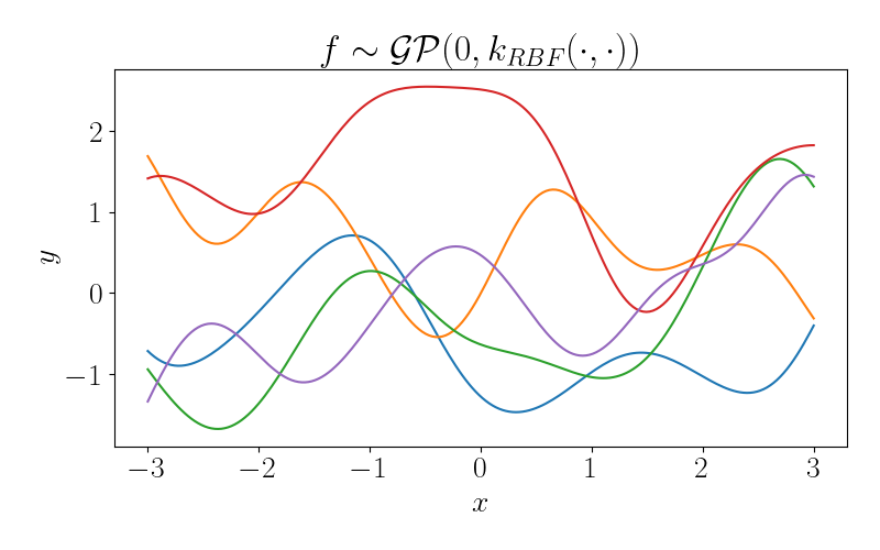
We can see that each of these functions is very smooth, with similarity between nearby points in the domain smoothly decaying as the distance between them increases.
However, in many cases this smoothness assumption isn’t warranted. For example, consider the data below, where the gray line is the true (noiseless) function, and the dots represent (noisy) observations of this function.
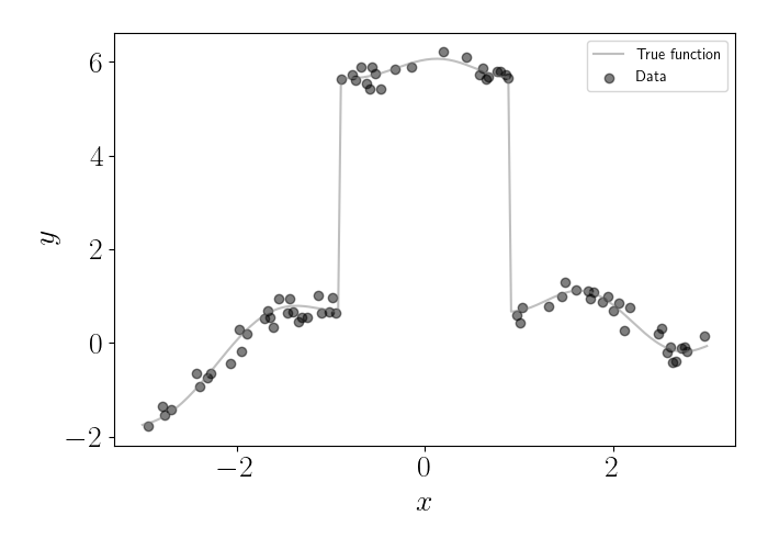
In this dataset, there’s a large discontinuity around $x=0.$ Clearly, this is a non-smooth function in that region of the domain. If we were to fit a GP with an RBF kernel, we would get the posterior plotted below in red.
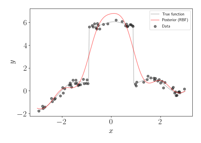
We can see that the RBF kernel tends to over-smooth the region with the discontinuity. This is due to the fact that the RBF kernel is assuming a gradual decay in similarity between points as they move farther apart. For this type of situation, we might consider a different type of covariance function; specifically, we want one that can model jumps like this one. This is one of the major use cases of the Matérn family of covariance functions, which we explore next.
Matérn kernels
The Matérn family of kernels were popularized by Michael Stein, who coined the name based on initial work by statistician Bertil Matérn. Matérn was originally interested in analyzing the spatial organization of forests and proposed several covariance functions for these problems. These covariance functions have found lots of utility outside of forestry and spatial analysis since then.
The form of the Matérn class of functions is given by
\[k_M(x, x^\prime) = \frac{2^{1 - \nu}}{\Gamma(\nu)} \left( \frac{\sqrt{2 \nu} |x - x^\prime|}{\ell} \right)^\nu K_\nu \left( \frac{\sqrt{2 \nu} |x - x^\prime|}{\ell} \right)\]where $\ell$ is a length-scale parameter, $\nu$ is a positive parameter, and $K_{\nu}$ is a modified Bessel function. The $\nu$ parameter effectively controls the level of smoothness of the function. As $\nu \to \infty$, we recover exactly the RBF kernel. For lower values of $\nu$, we obtain rougher functions. In general, a GP with a Matérn kernel with parameter $\nu$ is $\lceil \nu \rceil - 1$ times differentiable.
When $\nu$ is a half-integer (that is, $\nu = d + \frac12$ for any $d \in \mathbb{N}_+$), the kernel has an especially nice form as the product of an exponential function and a polynomial function of order $d$. Three of the most popular choices are $\nu \in \{\frac12, \frac32, \frac52\}.$ The form of the kernel function for these values of $\nu$ are below.
\begin{align} k_{M}^{1/2}(x, x^\prime) &= \exp\left( - \frac{|x - x^\prime|}{\ell} \right) \\ k_{M}^{3/2}(x, x^\prime) &= \left( 1 + \frac{\sqrt{3} |x - x^\prime|}{\ell} \right) \exp\left( - \frac{\sqrt{3} |x - x^\prime|}{\ell} \right) \\ k_{M}^{5/2}(x, x^\prime) &= \left( 1 + \frac{\sqrt{5} |x - x^\prime|}{\ell} + \frac{5 (x - x^\prime)^2}{3 \ell^2} \right) \exp\left( - \frac{\sqrt{5} |x - x^\prime|}{\ell} \right) \end{align}
Note that, while we can think of $\ell$ as a parameter as in the RBF kernel, we often fix $\nu$ before performing inference. While it’s common to optimize the length-scale parameter during inference, it’s more difficult to optimize $\nu$ due to computational infeasibility and the extreme changes in the functions that occur as $\nu$ changes. For this reason, we’ll denote the Matérn kernel indexed by $\nu$ as $k_{M}^{\nu}(\cdot, \cdot).$ We will explore these effects more below.
Below, we plot several functions drawn from a GP with a Matérn kernel with the $\nu$ parameter varied.
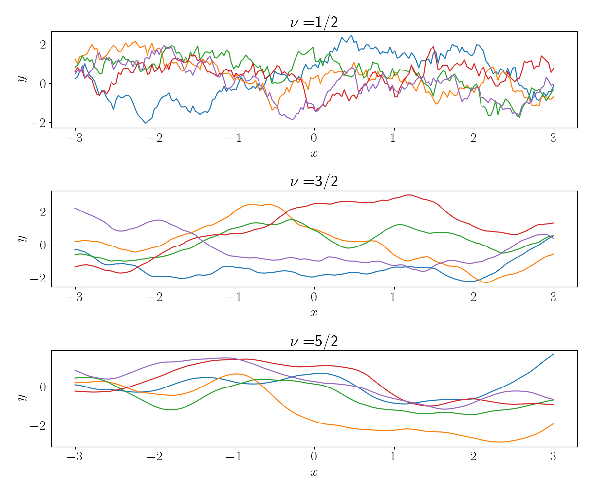
When $\nu = \frac12$, we can see that the sampled functions are zero times differentiable. In fact, we see that there are very sharp jumps in the functions. As $\nu$ increases, we see that the functions become smoother, with $\nu=\frac52$ already resembling functions drawn using the RBF kernel.
Now, let’s return to our regression example from above. This time, let’s fit a GP using a Matérn kernel with $\nu = \frac32.$ Below is the GP posterior. Below, we plot the posterior for this GP in green, along with the posterior for the GP with an RBF kernel in red.
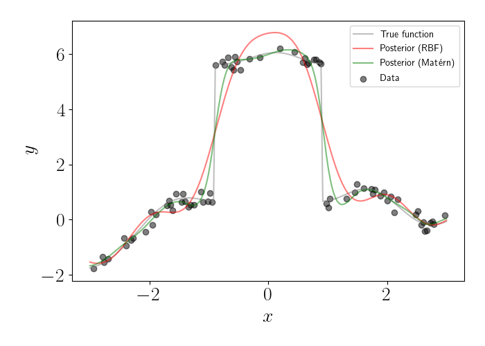
We can see that the Matérn kernel is able to better capture the sharp jump in the function (although it’s not perfect). The RBF kernel oversmooths this discontinuity, and actually “overshoots” the jump in the middle. Meanwhile, both kernels perform well outside of this jump, where the function is smooth.
References
- Rasmussen, Carl Edward. “Gaussian processes in machine learning.” Summer school on machine learning. Springer, Berlin, Heidelberg, 2003.
- Stein, Michael L. Interpolation of spatial data: some theory for kriging. Springer Science & Business Media, 2012.
- Matérn, Bertil. Spatial variation. Vol. 36. Springer Science & Business Media, 2013.