Andy Jones
Linear model of coregionalization
\(\DeclareMathOperator*{\argmin}{arg\,min}\) \(\DeclareMathOperator*{\argmax}{arg\,max}\)
Gaussian process primer
Recall that a Gaussian process (GP) can be viewed as a prior distribution for a function $f : \mathbb{R}^P \rightarrow \mathbb{R}$. Here, we assume that we have a set of $P$-dimensional inputs arranged in a matrix $\mathbf{X} \in \mathbb{R}^{P \times N}$ and a scalar output in a vector $\mathbf{y} \in \mathbb{R}^N$. A GP is parametrized by a mean and kernel function $k : \mathbb{R}^P \times \mathbb{R}^P \rightarrow \mathbb{R}$. Without loss of generality, we’ll assume the mean is zero.
The GP regression model with noisy outputs can be written as
\[y_i = f(\mathbf{x}_i) + \epsilon,~~~f \sim \mathcal{GP}(0, k(x_i, x^\prime)).\]Equivalently, we can write the model is term of a multivariate normal:
\[\mathbf{y} \sim \mathcal{N}(\mathbf{0}, \mathbf{K}_{XX} + \sigma^2 \mathbf{I}_N)\]where $\mathbf{0}$ is a vector of all zeros, and $\mathbf{K}_{XX}$ is a $N \times N$ matrix containing the kernel’s evaluation at all pairs of input points.
We can then make predictions based on the model by leveraging the properties of the conditional multivariate normal. Suppose we have a new set of input points arranged in a $P \times M$ matrix $\mathbf{X}^\star$. The distribution of the corresponding noiseless outputs $\mathbf{f}^\star \in \mathbb{R}^M$ is then
\[\mathbf{f}^\star | \mathbf{y}, \mathbf{X}, \mathbf{X}^\star \sim \mathcal{N}(\mu, \Sigma)\]where
\[\mu = \mathbf{K}_{\mathbf{X}^\star \mathbf{X}} \mathbf{K}_{\mathbf{X}\mathbf{X}}^{-1} \mathbf{y},~~~\Sigma = \mathbf{K}_{\mathbf{X}^\star \mathbf{X}^\star} - \mathbf{K}_{\mathbf{X}^\star \mathbf{X}} \mathbf{K}_{\mathbf{X} \mathbf{X}}^{-1} \mathbf{K}_{\mathbf{X} \mathbf{X}^\star}.\]Given this foundation for GPs, we next turn to multi-output GPs and the linear model of coregionalization.
Multi-output GPs
Traditional GPs (as above) only allow for a single scalar output. However, we often are interested in understanding the relationship between the input and multiple outputs. That is, if we suppose we have $Q$ output dimensions, we would like to place a prior on a function $f : \mathbb{R}^P \rightarrow \mathbb{R}^Q$.
One straightforward way to do this would be to using $Q$ separate independent GPs to model each of the outputs separately. However, this approach ignores any correlation that may exist in the outputs.
Several approaches have been developed for more sophisticated modeling of this multi-output function. Here, we’ll review the linear model of coregionalization (LMC).
Linear model of coregionalization
To model the association between the outputs, the LMC assumes we have $L$ shared latent Gaussian processes $f_1, \dots, f_L$, where typically $L < Q$. The model for sample $i$ is then:
\begin{align} \mathbf{y}_i &= \mathbf{W} \textbf{f}_i + \epsilon \\ \text{f}_{i\ell} &= f_\ell(\mathbf{x}_i) \\ f_\ell &\sim \mathcal{GP}(\mathbf{0}, \mathbf{K}_{\ell}) \\ \epsilon &\sim \mathcal{N}(\mathbf{0}, \sigma^2 \mathbf{I}_Q). \end{align}
Here, $\textbf{f}_i$ is a vector of $L$ latent funciton evaluations for sample $i$, and $\mathbf{W} \in \mathbb{R}^{P \times L}$ is a “loadings” matrix mapping from the latent function values to the observed data outputs. $\mathbf{K}_\ell$ is the $\ell$th kernel function evaluated at all pair of points.
Notice that the distribution of $\textbf{f}_\ell$ will be Gaussian (by the definition of a GP):
\[\textbf{f}_\ell \sim \mathcal{N}(\mathbf{0}, \mathbf{K}_\ell).\]Furthermore, we know that a linear combination of Gaussians will still be Gaussian, so the outputs will also be Gaussian. The covariance between two outputs $y_{iq}$ and $y_{jq^\prime}$ will be given by
\[\text{cov}(y_{iq}, y_{jq^\prime}) = \sum\limits_{\ell=1}^L k_\ell(\mathbf{x}_i, \mathbf{x}_j) w_{q\ell} w_{q^\prime \ell}\]where $w_{q\ell}$ is the element of the loadings matrix $\mathbf{W}$ on row $q$ and column $\ell$. Putting all of this information together, we can write the distribution of $\mathbf{Y}$ as one big multivariate normal distribution:
\[\text{vec}(\mathbf{Y}) \sim \mathcal{N}(\mathbf{0}, \boldsymbol{\Sigma} + \sigma^2 \mathbf{I}_{NQ}),~~~\boldsymbol{\Sigma} = \sum\limits_{\ell=1}^L \mathbf{K}_{\ell} \otimes \mathbf{w}_\ell\mathbf{w}_\ell^\top\]where $\otimes$ denotes a Kronecker product and $\text{vec}(\cdot)$ is the vectorization function:
\[\text{vec}(\mathbf{Y}) = \begin{bmatrix} \mathbf{y}_1 \\ \mathbf{y}_2 \\ \vdots \\ \mathbf{y}_N \end{bmatrix} \in \mathbb{R}^{NQ}.\]Note that if each latent GP has the same kernel function, then the covariance function simplifies as
\[\boldsymbol{\Sigma} = \mathbf{K} \otimes \mathbf{W} \mathbf{W}^\top.\]Thus, we now have a way to model correlation between the outputs. This correlation is captured in the matrix $\mathbf{W}$. While we can still model nonlinear functions through our latent GPs, the top level of the model is a simple linear model (a linear function of the GP function evaluations).
Example
Suppose we have a one dimensional input $\mathbf{x} \in \mathbb{R}^N$ and a two-dimensional output $\mathbf{Y} \in \mathbb{R}^{N \times Q}$. Below is a plot of the data, where the plot “Y1” corresponds to the first output dimension and “Y2” corresponds to the second output.
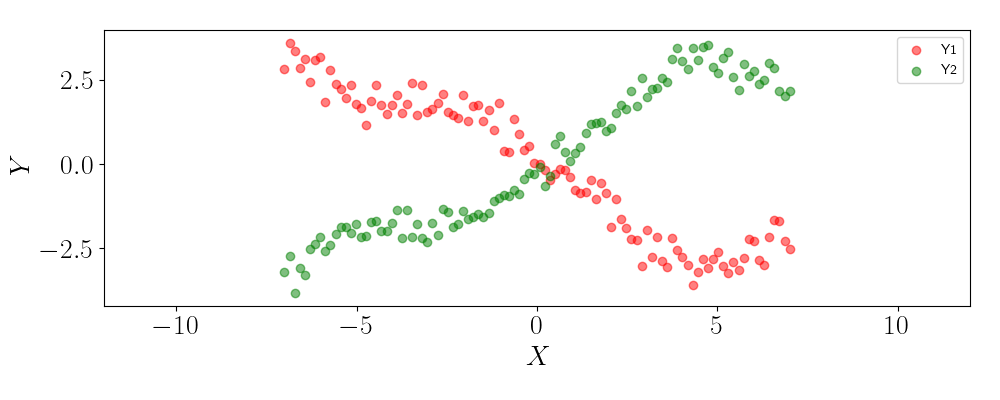
We can see that the two outputs are highly (inversely) correlated with one another. This correlation should allow us to share strength across the outputs in our predictions, rather than treating each of the outputs as independent.
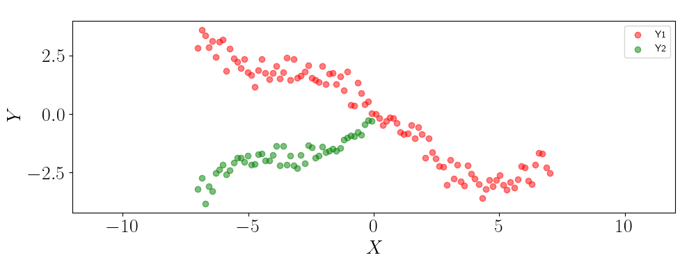
To show this, let’s suppose that we only observe half of the samples for the second output, and we’d like to predict the output for the remaining half. Below is a plot of the observed data.
Let’s look at what happens if we use two independent GPs to make predictions. Below, we show the GP predictions for the second output on the missing values.
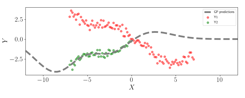
We can see that the GP predictions revert back to zero as we move right across the plot. This behavior is due to the fact that the GP is unable to leverage any information in the values for Y1.
Now, let’s see what happens when we fit an LMC. Here, we’ll set $L=1$ so that there’s one latent GP, but the outputs are linearly correlated based on this latent GP. In this case, we must learn the values for $\mathbf{W}$, which is a vector of length two in this case. Below are the predictions for the LMC in the solid black line:
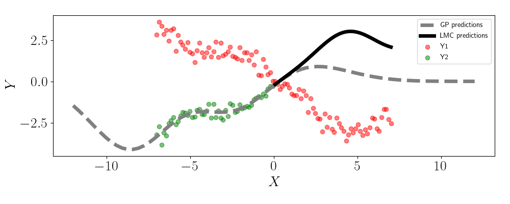
We can see that the predictions for Y2 maintains the correlation seen in the data that’s observed for both outputs. This stands in contrast to the single-output GP, which simply reverts to the GP prior.
Code
The code for the example can be found in my GitHub repository for the post.
References
- Goulard, Michel, and Marc Voltz. “Linear coregionalization model: tools for estimation and choice of cross-variogram matrix.” Mathematical Geology 24.3 (1992): 269-286.
- Mauricio Alvarez’s slides on multi-output GPs.
- GPFlow’s example on coregionalization models.