Andy Jones
Unifying linear dimensionality reduction methods
Linear dimensionality reduction is a cornerstone of machine learning and statistics. Here we review a 2015 paper by Cunningham and Ghahramani that unifies this zoo by casting each of them as a special case of a very general optimization problem.
The space of linear dimensionality reduction methods is enormous. Developing a unified framework for understanding these methods can help draw connections between them and ultimately improve them. Here, we review the general optimization framework proposed by Cunningham and Ghahramani, and focus on three important cases: PCA, LDA, and CCA.
Linear dimensionality reduction
To start, we give a formal definition of linear dimensionality reduction as written by Cunningham and Ghahramani.
Definition (Linear dimensionality reduction). Given a data matrix $X \in \mathbb{R}^{p \times n}$ containing $n$ data points, $X = \begin{bmatrix} x_1, \dots, x_n \end{bmatrix}$, and a specified target dimensionality $k < p$, a linear dimensionality reduction method optimizes a function $f_X(M)$ with respect to $M$ to produce a linear transformation (matrix) $P$ such that the reduced data matrix is given by $Y = PX \in \mathbb{R}^{k \times n}$ where $P$ is a constant function of $M$.
Clearly, this definition is very general. Essentially, a linear dimensionality reduction method is one that finds a linear mapping to a lower dimensional space according to some criteria.
Linear dimensionality reduction as an optimization problem
Cunningham and Ghahramani assert that all linear dimensionality reduction methods can be cast as the following optimization problem. \begin{align} &\text{minimize } f_X(M) \\ &\text{subject to } M \in \mathcal{M} \end{align} where $\mathcal{M}$ is a matrix manifold.
There are two common choices for the matrix manifold $\mathcal{M}$:
- All rank $k$ linear mappings. That is, $\mathcal{M} = \mathbb{R}^{p \times k}$. This is the simplest case, where $M$ is unconstrained.
- Matrices with orthogonal columns. That is, $\mathcal{M} = \{M \in \mathbb{R}^{p \times k} : M^\top M = I_p\}$. This set is often denoted $\mathcal{M} = \mathcal{O}^{p \times k}$. This is perhaps the more common assumption and shows up in the most popular dimensionality reduction methods — like PCA, which we review next.
Principal component analysis (PCA)
PCA has been formulated in many equivalent ways. Two of the most common frameworks are the “variance maximization” perspective and the “reconstruction error minimization” perspective.
We can write both of these formulations in terms of the program above. The variance maximization perspective casts the PCA objective as finding the vectors in data space that, when the data is projected onto these vectors, maximize the variance of the resulting projections. To see this, note that given a vector $v \in \mathbb{R}^p$, the projection of $X$ onto this vector is given by $X^\top v$. Without loss of generality, we can assume that the data is mean-centered, which implies that the variance of this projection is given by
\[\text{var}(X^\top v) = (X^\top v)^\top X^\top v = v^\top XX^\top v\]where $XX^\top$ is the sample covariance. Thus, for PCA with $k=1$ the optimization function we wish to minimize is the negative variance,
\[f_X(v) = -v^\top XX^\top v.\]When $k>1$, we wish to find a set of vectors $M = \begin{bmatrix} v_1, \dots, v_k \end{bmatrix}$ that maximize the overall variance,
\[f_X(M) = -\sum\limits_{j=1}^k v_j^\top XX^\top v_j = -\text{tr}(M^\top XX^\top M).\]Writing out the full optimization program, we have
\begin{align} &\text{minimize } -\text{tr}(M^\top XX^\top M) \\ &\text{subject to } M \in \mathcal{O}^{p \times k}. \end{align}
The “reconstruction error minimization” perspective yields a slightly different but very similar form (and identical solution). Again, starting with $k=1$ our goal from this point-of-view is to find a vector $v \in \mathbb{R}^k$ such that when $X$ is linearly compressed using this vector, then uncompressed, the reconstruction error is minimized. We can think of the linear operation $v^\top X$ as compressing each data point to one dimension. Then, we can project these compressed data points back up to $p$ dimensions by premultiplying by $v$,
\[\widehat{X} = v v^\top X.\]Again, the extension to $k>1$ is straightforward, and we have the following optimization program:
\begin{align} &\text{minimize } \|X - MM^\top X\|_2 \\ &\text{subject to } M \in \mathcal{O}^{p \times k}. \end{align}
The solution to both of these optimization problems is given by a singular value decomposition. Recall the Eckart-Young theorem:
Theorem (Eckart-Young, 1936). The minimizer of $\|X - \widehat{X}\|_2$ such that $\text{rank}(\widehat{X}) \leq k$ is given by a singular value decomposition of $X.$ In particular, $\widehat{X}^\star = U_k D_k V_k^\top$ where $D_k = \text{diag}(\sigma_1, \dots, \sigma_k)$ contains the top $k$ singular values, and $U_k$ and $V_k$ contain the corresponding left and right singular vectors.
We can summarize the data in terms of its sample covariance matrix $\Sigma = XX^\top$, which implies that
\[\Sigma = U_k D_k V_k^\top (U_k D_k V_k^\top)^\top = U_k D_k V_k^\top V_k D_k U_k^\top.\]Using the orthogonality of $V_k$, we have
\[\Sigma = U_k D_k^2 U_k^\top = Q_k \Lambda_k Q_k^\top\]where $\Lambda_k = \text{diag}(\lambda_1, \dots, \lambda_k)$ contains the top $k$ eigenvalues of $\Sigma$, and $Q_k$ contains the corresponding eigenvectors.
Linear discriminant analysis (LDA)
We can also consider dimensionality reduction in the context of classification. LDA is perhaps the simplest way of doing so.
In addition to our data $X$, suppose we have class labels $\{\ell_1, \dots, \ell_n\}$, where $\ell_i \in \{1, \dots, C\}$. Here, $C$ is the total number of classes.
LDA seeks a hyperplane that minimizes the total variance of the data within each class, while maximizing the variance between classes. The covariances within each class $\Sigma_W$ and between classes $\Sigma_B$ are given by
\[\Sigma_W = \sum\limits_{i=1}^n (x_i - \mu_{\ell_i}) (x_i - \mu_{\ell_i})^\top,~~~~~\Sigma_B = \sum\limits_{c=1}^C (\mu_c - \mu_X) (\mu_c - \mu_X)^\top\]where $\mu_c$ is the mean of class $c$, and $\mu_X$ is the overall data mean. Notice that the sum of these two covariance terms will equal the overall data covariance:
\begin{align} &\sum\limits_{i=1}^n (x_i - \mu_{\ell_i}) (x_i - \mu_{\ell_i})^\top + \sum\limits_{i=1}^n (\mu_{\ell_i} - \mu_X) (\mu_{\ell_i} - \mu_X)^\top \\ =& \sum\limits_{i=1}^n (x_i - \mu_X) (x_i - \mu_X)^\top \\ =& \Sigma. \end{align}
We again begin by considering the case when $k=1$. In this case, the optimization problem of LDA is to find a vector $v$ that maximizes the the ratio of the two types of implied variance (equivalently, minimize the negative ratio):
\[\text{minimize } -\frac{v^\top \Sigma_W v}{v^\top \Sigma_B v}.\]The generalization to $k>1$ is straightforward:
\begin{align} &\text{minimize } -\frac{\text{tr}(M^\top \Sigma_W M)}{\text{tr}(M^\top \Sigma_B M)} \\ &\text{subject to } M \in \mathcal{O}^{p \times k}. \end{align}
Canonical correlation analysis (CCA)
The general goal of CCA is to find shared patterns of variation across two datasets with shared samples (but different features). In particular, we assume we have two data matrices $X_a \in \mathbb{R}^{p_a \times n}$ and $X_b \in \mathbb{R}^{p_b \times n}$. The goal is to find linear mappings of each of the datasets such that their low-dimensional representations are maximially correlated.
Starting with the $k=1$ case, we seek linear mappings $P_a \in \mathbb{R}^{p_a}, P_b \in \mathbb{R}^{p_b}$ that map the data to low-dimensional representations $y_a = P_a^\top X_a, y_b = P_b^\top X_b$. We then want to optimize $P_a$ and $P_b$ to maximize the Pearson correlation coefficient between $y_a$ and $y_b$.
\[\min_{P_a, P_b} -\frac{y_a^\top y_b}{\sqrt{y_a^\top y_a y_b^\top y_b}} = -\frac{X_a^\top P_a P_b^\top X_b}{\sqrt{X_a^\top P_a P_a^\top X_a X_b^\top P_b P_b^\top X_b}}.\]Moving to the more general case with $k>1$, we now have two matrices $P_a \in \mathbb{R}^{k \times p_a}, P_b \in \mathbb{R}^{k \times p_b}$. In this case, CCA adds additional constraints that the low-dimensional representations are uncorrelated and have unit variance, as well as requiring a diagonal cross-covariance between them. In particular, the optimization program becomes
\begin{align} &\text{minimize } \frac{\text{tr}(Y_a Y_b^\top)}{\sqrt{\text{tr}(Y_a Y_a^\top) \text{tr}(Y_b Y_b^\top)}} = \frac{\text{tr}(P_a X_a X_b^\top P_b^\top)}{\sqrt{\text{tr}(P_a X_a X_a^\top P_a^\top) \text{tr}(P_b X_b X_b^\top P_b^\top)}} \\ &\text{subject to } \frac1n P_a X_a X_a^\top P_a^\top = I \\ &\hspace{24mm}\frac1n P_b X_b X_b^\top P_b^\top = I \\ &\hspace{24mm}P_a X_a X_b^\top P_b^\top = \Lambda = \text{diag}(\lambda_1, \dots, \lambda_k) \end{align} where $\Lambda$ is some diagonal matrix.
We can reparameterize this in terms of orthogonal matrices $M_a \in \mathcal{O}^{p_a \times k}, M_b \in \mathcal{O}^{p_b \times k}$. Specifically, let
\begin{align} P_a &= M_a^\top (X_a X_a^\top)^{-1/2} \\ P_b &= M_b^\top (X_b X_b^\top)^{-1/2}. \end{align}
Plugging this into the CCA objective, we have
\begin{align} &\frac{\text{tr}(M_a^\top (X_a X_a^\top)^{-1/2} X_a X_b^\top (X_b X_b^\top)^{-1/2} M_b)}{\sqrt{\text{tr}(M_a^\top (X_a X_a^\top)^{-1/2} X_a X_a^\top (X_a X_a^\top)^{-1/2} M_a) \text{tr}(M_b^\top (X_b X_b^\top)^{-1/2} X_b X_b^\top (X_b X_b^\top)^{-1/2} M_b)}} \\ =& \frac{\text{tr}(M_a^\top (X_a X_a^\top)^{-1/2} X_a X_b^\top (X_b X_b^\top)^{-1/2} M_b)}{\sqrt{\text{tr}(M_a^\top M_a) \text{tr}(M_b^\top M_b)}} \\ =& \text{tr}(M_a^\top (X_a X_a^\top)^{-1/2} X_a X_b^\top (X_b X_b^\top)^{-1/2} M_b). \end{align}
Notice that the optimization program’s constraints are automatically satisfied by restricting $M_a$ and $M_b$ to the Stiefel manifold:
- $P_a X_a X_a^\top P_a^\top = M_a^\top (X_a X_a^\top)^{-1/2} X_a X_a^\top (X_a X_a^\top)^{-1/2} M_a = M_a^\top M_a = I$
- $P_b X_b X_b^\top P_b^\top = M_b^\top (X_b X_b^\top)^{-1/2} X_b X_b^\top (X_b X_b^\top)^{-1/2} M_b = M_b^\top M_b = I$
- $M_a^\top (X_a X_a^\top)^{-1/2} X_a X_b^\top (X_b X_b^\top)^{-1/2} M_b = M_a^\top \Lambda_a \Lambda_b M_b = \Lambda M_a^\top M_b = \Lambda.$
However, even though we restricted $M_a$ and $M_b$ to be orthogonal, this doesn’t imply that the original $P_a$ and $P_b$ are orthogonal. To address this, some people use post hoc corrections on $P_a, P_b$ to make them orthogonal.
Another route is to directly require orthogonality as part of the original optimization program. Specifically, using the general approach of Cunningham and Ghahramani, we can instead write the program as follows.
\begin{align} &\text{minimize } \frac{\text{tr}(M_a^\top X_a X_b^\top M_b)}{\sqrt{\text{tr}(M_a^\top X_a X_a^\top M_a) \text{tr}(M_b^\top X_b X_b^\top M_b)}} \\ &\text{subject to } M_a \in \mathcal{O}^{p_a \times k} \\ &\hspace{24mm}M_b \in \mathcal{O}^{p_b \times k}. \end{align}
Clearly, this program fits into the general framework, so we can use the same generic optimization methods here.
Optimization
The similarities among all of these linear dimensionality reduction methods motivates a general-purpose optimization scheme. When the matrix $M$ is unconstrained, we can use general first- and second-order methods.
The case where $M$ is constrained to the Stiefel manifoldis is more difficult. Standard gradient-based optimization methods will quickly veer off of the desired manifold. With the constraint $M \in \mathcal{O}^{p \times k}$, we need to make sure that the estimate at every step, $M^{(t)}$, remains on the manifold.
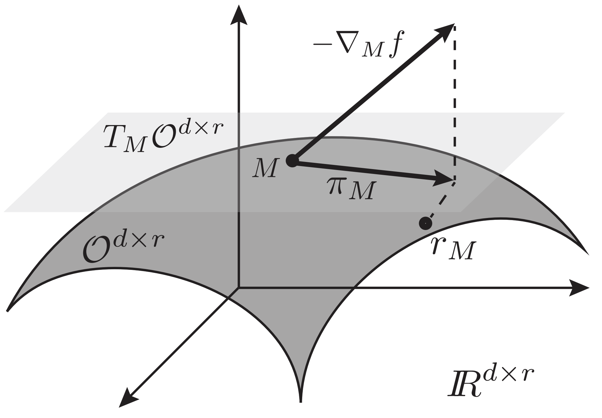
Cunningham and Ghahramani propose a projected gradient descent method for this setting. The basic idea is to take a step in the direction of the negative gradient (as in typical gradient descent), but then project back onto the desired manifold. Here, a projection means that we place our estimate at the closest point on the manifold.
Unfortunately, finding the closest point on the Stiefel manifold from an arbitrary point in $\mathbb{R}^{p \times k}$ is nontrivial. For this reason, the projection is broken down into two steps: projection onto the tangent space and retraction onto the Stiefel manifold.
A simplified sketch of the algorithm (ignoring step sizes) goes as follows.
- $g = \nabla_M f(M)~~~~~~~~~~~~~$ (Calculate gradient)
- $Z = \pi_M(\nabla_M f(M))~~~$ (Project onto tangent space)
- $M^{(t+1)} = r_M(Z)~~~~~~~~$ (retract onto manifold)
The algorithm above can be used as a black-box algorithm for finding solutions to linear dimensionality reduction methods that are constrained to the Stiefel manifold. These steps can be visualized below.
Conclusion
In the current era of fancy nonlinear methods, linear dimensionality reduction methods are often overlooked. However, these methods provide a necessary foundation for more complicated approaches. Moreover, developing a unified view of these approaches strengthens their flexibility and usefuless. A common framework allows us to share algorithms, notation, and extensions across all members of the family, rather than viewing these methods as a scattering of ad hoc cases.
References
- Cunningham, John P., and Zoubin Ghahramani. “Linear dimensionality reduction: Survey, insights, and generalizations.” The Journal of Machine Learning Research 16.1 (2015): 2859-2900.