Andy Jones
Visualizing Lebesgue integration
\(\DeclareMathOperator*{\argmin}{arg\,min}\) \(\DeclareMathOperator*{\argmax}{arg\,max}\)
Analogous to approximating Riemannian integrals with “tall and narrow” rectangles under the curve, Lebesgue integrals can be approximated with “short and wide” rectangles. We visualize both of these concepts here.
Riemannian integration
Recall the construction of a Riemannian integral via infinitesimal sums. Consider the integral of a function $f(x)$ on the interval $[a, b]$:
\begin{equation} \int_a^b f(x) dx. \label{eq:1} \tag{1} \end{equation}
An intuitive interpretation of this Riemannian integral is that its value is equal to the area underneath the curve $f(x).$ To approximate this area, we can break the domain into small intervals of width $dx$; form a rectangle on each interval whose height is equal to the function at that point; and sum the total area of the rectangles along the interval $[a, b].$
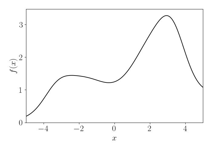
For example, consider the function below on the interval $[-5, 5].$
As a coarse approximation, consider splitting the domain into intervals of size $dx=0.5.$ Below, we draw a rectangle above each subinterval, connecting its top left corner with the function $f(x).$ Because the area of a rectangle is simple to compute, we could use this as a rough approximation to the integral in Equation \ref{eq:1}.
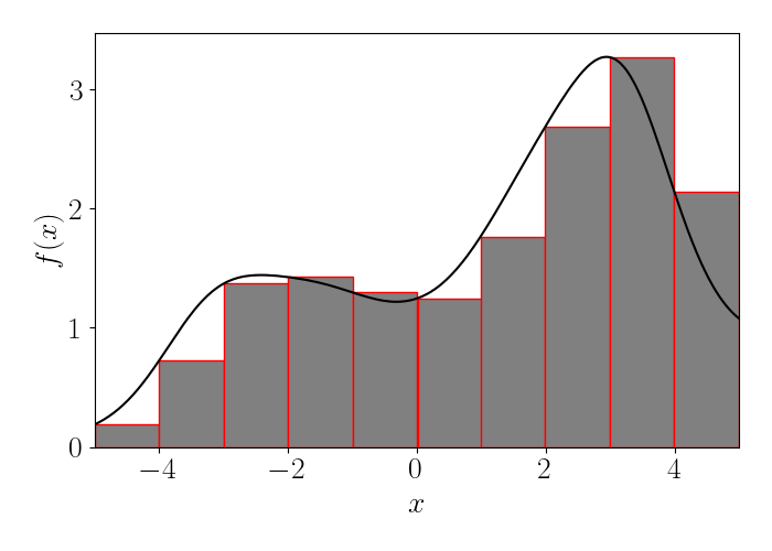
However, it’s clear that this approximation will be relatively poor, especially for functions with high curvature. We can always improve the approximation by decreasing the width $dx$ of the subintervals. The animation below, shows a sequence of approximations with decreasing $dx.$
In the limit as $dx \to 0,$ we obtain the definition of the original full integral.
Lebesgue integration
We can visualize the Lebesgue integral in a similar way, except that our rectangles will be “flipped sideways” this time. Recall that the Lebesgue integral of a function $f(x)$ with respect to the measure $\mu$ over a set $E$ is denoted as
\[\int_E f(x) d \mu(x) = \int_E f d \mu,\]where the above forms are two equivalent ways to denote the same integral. There are several equivalent definitions and constructions of the Lebesgue integral. One interesting one for our purposes is to define it in terms of an improper Riemannian integral. For our purposes, suppose $f$ is a nonnegative function. Then we have
\[\int_E f d \mu = \int_0^\infty f^*(t) dt,\]where $f^*$ is defined as
\[f^*(t) = \mu\left(\{ x \in E | f(x) > t \}\right).\]We can visualize this as slicing the function along horizontal cross sections (whereas we can think of the Riemannian integral as taking vertical slices; see the above figures).
Specifically, consider drawing boxes with height $dt,$ where the box corresponding to a value $t$ only spans the regions of the domain such that $\{ x \in E | f(x) > t \}.$ Importantly, this implies that each box may be disconnected horizontally. For example, consider the visualization below, where we use the same function $f$ as in our Riemannian integral example.
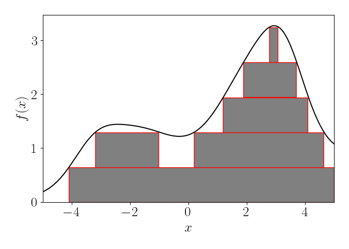
In the above plot, each horizontal box corresponds to one cross section of the function. If $\mu$ is the Lebesgue measure here, we obtain another route to arrive at the same integral as the Riemannian case. In particular, in the limit that the height of the boxes $dt \to 0.$ The animation below shows this.
One of the primary benefits of the Lebesgue integral, of course, is its ability to generalize to other measures (even discrete ones). But with the simple setting in a subset of the real line that we saw in this post, we can build intuition about its benefits.
References
- Wikipedia page on Lebesgue integration.