Linear discriminant analysis from scratch

In this post, we’ll review a family of fundamental classification algorithms: linear and quadratic discriminant analysis.

Disciminative classifiers

Consider a classification setting in which we’re given data $\mathbf{X}$ and labels $\mathbf{Y}$ that come from $K$ disjoint categories, and we’re tasked with finding the best way to separate the data into their respective classes based on the data $\mathbf{X}$. One way to approach this problem is to estimate a conditional probability for each class. Then, when we want to predict the class of a new point, we can choose the class that has the maximum probability given the data point. The conditional probability for data point $i$ belonging to class $k$ is denoted

By a simple application of Bayes rule, we have

\begin{align} \mathbb{P}[Y_i = k | X_i] &= \frac{\mathbb{P}[X_i | Y_i = k] \mathbb{P}[Y_i = k]}{\mathbb{P}[X_i]} \\ &= \frac{\mathbb{P}[X_i | Y_i = k] \mathbb{P}[Y_i = k]}{\sum\limits_{k=1}^K \mathbb{P}[X_i | Y_i = k] \mathbb{P}[Y_i = k]} \\ &\propto \mathbb{P}[X_i | Y_i = k] \mathbb{P}[Y_i = k] \end{align}

Here, $\mathbb{P}[X_i | Y_i = k]$ is the likelihood, $\mathbb{P}[Y_i = k]$ is the prior probability of a point belonging to class $k$, and $\mathbb{P}[X_i]$ is the evidence.

If we know the likelihood and the prior upfront (or we can estimate them), then we can classify points with the decision rule $D$:

Quadratic discriminant analysis

Consider the case where we assume the likelihood to be Gaussian:

Recall that the Gaussian PDF is

Denote the prior for class $k$ as $\pi_k = \mathbb{P}[Y_i = k]$. Then the conditional probability becomes

Taking the $\log$, we have

We can then apply the decision rule $\text{arg}\max_k \mathbb{P}[X_i | Y_i = k]$. Notice that the only term that depends on $x$ is $\frac12 (x - \mu_k)^\top \Sigma_k^{-1}(x - \mu_k)$. Thus, we can see that maximizing this decision criterion is is essentially finding the minimum distance between $X_i$ and each of the mean vectors $\mu_1, \dots, \mu_n$. However, this squared distance is scaled by the inverse covariance $\Sigma_k^{-1}$; this is called the Mahalanobis distance.

Also, notice that the objective $\frac12 (x - \mu_k)^\top \Sigma_k^{-1}(x - \mu_k)$ is quadratic in $x$, hence the name Quadratic Discriminant Analysis.

Linear discriminant analysis

If we assume that all classes have a common covariance matrix $\Sigma_k = \Sigma$, then the “distance” term becomes

\begin{align} \frac12 (x - \mu_k)^\top \Sigma_k^{-1}(x - \mu_k) &= \frac12 (x - \mu_k)^\top \Sigma^{-1}(x - \mu_k) \\ &= x^\top \Sigma^{-1} x - 2x^\top \Sigma^{-1} \mu_k + \mu_k^\top \Sigma^{-1} \mu_k. \end{align}

Notice that the term $x^\top \Sigma^{-1} x$ will be the same for all classes, and the term $\mu_k^\top \Sigma^{-1} \mu_k$ will be the same for all data points. Thus, the only term that affects the decision criterion in this case is $2x^\top \Sigma^{-1} \mu_k$. This is linear in $x$, thus the name “linear Discriminant analysis”.

To more explicitly define the linear function that separates the classes, consider the situation where $K = 2$. Observe that we will decide to classify a point into class $1$ if the following inequality holds:

\begin{align} \log \pi_1 - &\frac12 \log |\Sigma| - \frac12 (x - \mu_1)^\top \Sigma^{-1} (x - \mu_1) \\ &> \log \pi_2 - \frac12 \log |\Sigma| - \frac12 (x - \mu_2)^\top \Sigma^{-1} (x - \mu_2). \\ \end{align}

Otherwise, we categorize it as belonging to class 2.

Cancelling terms and doing some simple algebra (shown in detail here), we have

\begin{align} \log \pi_1 - \frac12 (x - \mu_1)^\top \Sigma^{-1} (x - \mu_1) &> \log \pi_2 - \frac12 (x - \mu_2)^\top \Sigma^{-1} (x - \mu_2) \\ - \frac12 (x - \mu_1)^\top \Sigma^{-1} (x - \mu_1) + \frac12 (x - \mu_2)^\top \Sigma^{-1} (x - \mu_2) &> \log \pi_2 - \log \pi_1 \\ \frac12 x^\top \Sigma^{-1} x + x^\top \Sigma^{-1} \mu_1 - \frac12 \mu_1^\top \Sigma^{-1} \mu_1 + \frac12 x^\top \Sigma^{-1} x - x^\top \Sigma^{-1} \mu_2 + \frac12 \mu_2^\top \Sigma^{-1} \mu_2 &> \log \pi_2 - \log \pi_1 \\ x^\top \Sigma^{-1} \mu_1 - x^\top \Sigma^{-1} \mu_2 &> \log \pi_2 - \log \pi_1 + \frac12 \mu_1^\top \Sigma^{-1} \mu_1 - \frac12 \mu_2^\top \Sigma^{-1} \mu_2 \\ x^\top \Sigma^{-1} (\mu_1 - \mu_2) &> \log \pi_2 - \log \pi_1 + \frac12 \mu_1^\top \Sigma^{-1} \mu_1 - \frac12 \mu_2^\top \Sigma^{-1} \mu_2 \\ \end{align}

In other words, the two classes are optimally divided by a hyperplane defined by the equation

Notice that, in terms of $x$, this is a linear function, where $x$ is weighted by the term $ \Sigma^{-1} (\mu_1 - \mu_2)$.

To estimate these parameters from data, we can take the most straightforward estimates:

LDA in Python

Putting this all together, LDA has a fairly straightforward implementation. Here’s mine, written in Python.

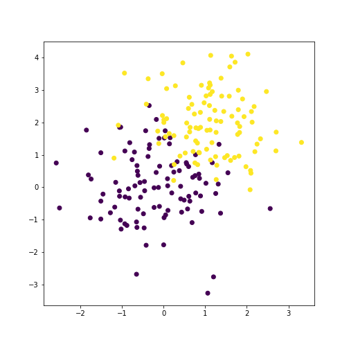
First, let’s generate some synthetic data:

import numpy as np
import matplotlib.pyplot as plt

# Generate data
mu1 = [0, 0]
mu2 = [1, 2]
cov = [[1, 0], [0, 1]]
n1 = 500
n2 = 50
n = n1 + n2
x1 = np.random.multivariate_normal(mean=mu1, cov=cov, size=n1)
x2 = np.random.multivariate_normal(mean=mu2, cov=cov, size=n2)
x = np.vstack([x1, x2])
y = np.concatenate([np.repeat(1, n1), np.repeat(2, n2)])

plt.scatter(x[:, 0], x[:, 1], c=y)
plt.show()

Now, we can estimate the priors, means, and covariances.

pi_hat_1 = n1 / n
pi_hat_2 = n2 / n

mu_hat_1 = 1 / n1 * np.sum(x1, axis=0)
mu_hat_2 = 1 / n2 * np.sum(x2, axis=0)

cov_hat_1 = 1 / (n1 - 1) * np.matmul((x1 - mu_hat_1).T, (x1 - mu_hat_1))
cov_hat_2 = 1 / (n2 - 1) * np.matmul((x2 - mu_hat_2).T, (x2 - mu_hat_2))
cov_hat = (cov_hat_1 + cov_hat_2) / 2

Let’s also define the log-likelihood function (to be evaluated at a single point).

def LL(x, mu, sigma, prior):
    dist = x - mu
    cov_inv = np.linalg.inv(sigma)
    cov_det = np.linalg.det(sigma)
    return -1/2 * np.log(2 * np.pi * cov_det) - 1/2 * np.matmul(np.matmul(dist.T, cov_inv), dist) + np.log(prior)

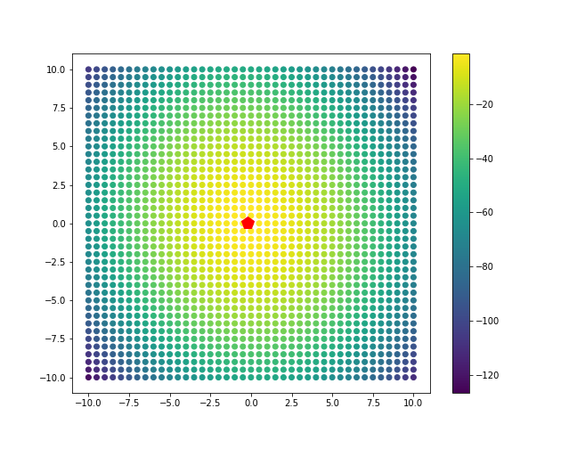
Now, let’s plot this log-likelihood for class 1 for a grid of points.

point_grid = np.mgrid[-10:10.1:0.5, -10:10.1:0.5].reshape(2, -1).T
ll_vals_1 = [LL(x, mu_hat_1, cov_hat, pi_hat_1) for x in point_grid]
ll_vals_2 = [LL(x, mu_hat_2, cov_hat, pi_hat_2) for x in point_grid]

plt.scatter(point_grid[:, 0], point_grid[:, 1], c=ll_vals_1)
plt.plot(mu_hat_1[0], mu_hat_1[1], 'rp', markersize=14)
plt.colorbar()
plt.show()

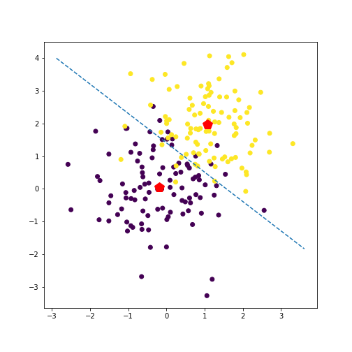
Let’s take a look at the inferred separating line.

def abline(slope, intercept):
    """Plot a line from slope and intercept"""
    axes = plt.gca()
    x_vals = np.array(axes.get_xlim())
    y_vals = intercept + slope * x_vals
    plt.plot(x_vals, y_vals, '--')
    
cov_inv = np.linalg.inv(cov_hat)

# slope
slope_vec = np.matmul(cov_inv, (mu_hat_1 - mu_hat_2))
slope = -slope_vec[0] / slope_vec[1]

# intercept
intercept_partial = np.log(pi_hat_2) - np.log(pi_hat_1) + 0.5 * np.matmul(np.matmul(mu_hat_1.T, cov_inv), mu_hat_1) - 0.5 * np.matmul(np.matmul(mu_hat_2.T, cov_inv), mu_hat_2)
intercept = intercept_partial / slope_vec[1]

# plotting
plt.scatter(x[:, 0], x[:, 1], c=y)
abline(slope, intercept)
plt.plot(mu_hat_1[0], mu_hat_1[1], 'rp', markersize=14)
plt.plot(mu_hat_2[0], mu_hat_2[1], 'rp', markersize=14)
plt.show()

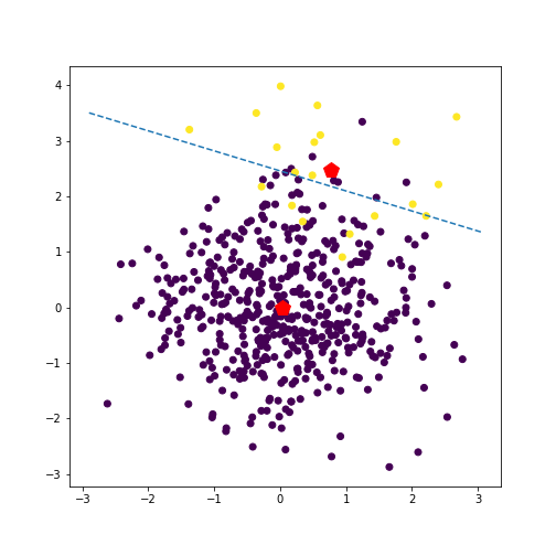
We can also investigate how this solution changes as we tweak certain aspects of the data and model.

For example, if we make one class much more prevalent than the other (say $n_1 = 500, n_2 = 20$), the prior favors this class, and the line subsequently moves closer to this class’s mean. See an example of this in the plot below.

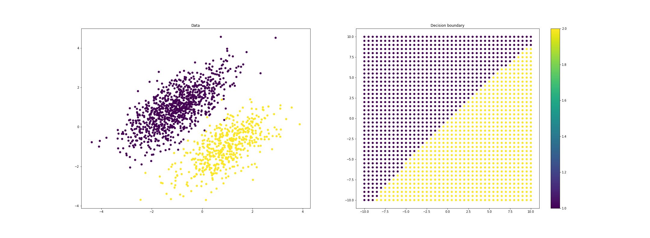
We can also investigate quadratic discriminant analysis, which can yield nonlinear decision boudnaries. For example, for imbalanced class sizes, the boundary will curve away from the larger class, favoring this class. Here’s a plot where we show the predicted class for a grid of points (blue is class 1, and yellow is class 2).

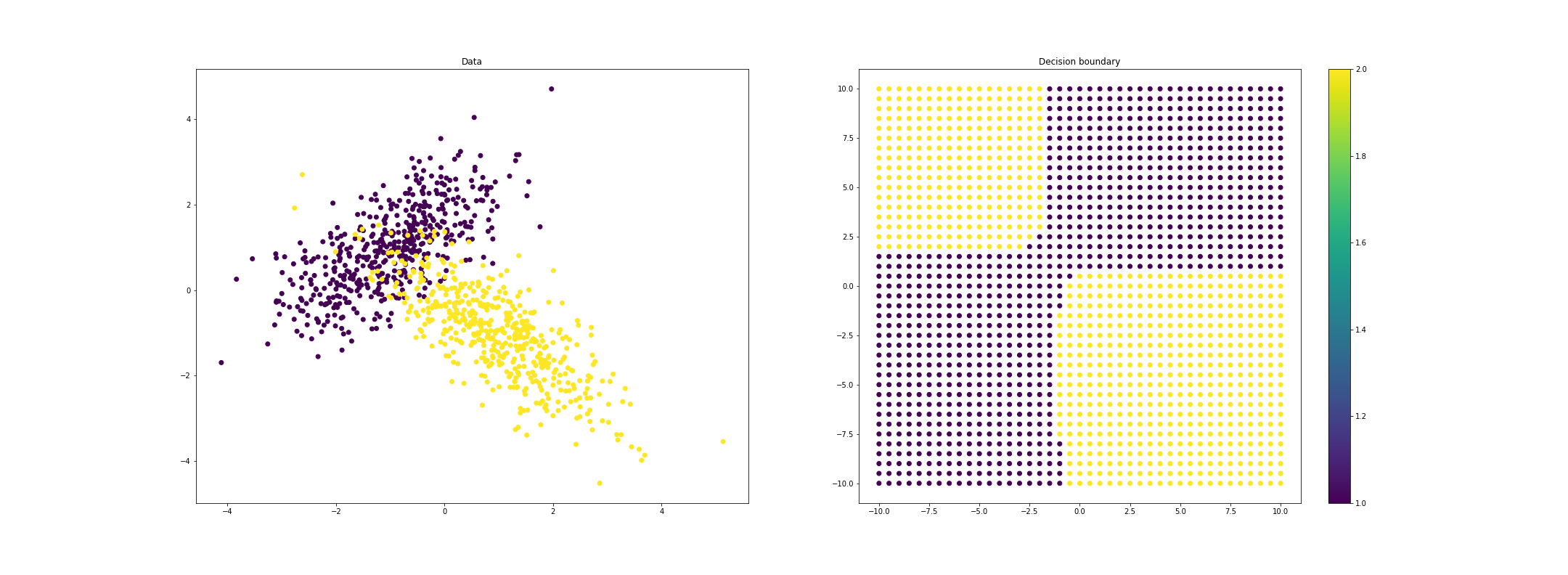
If we allow each class to have a unique covariance function, we can get even more highly nonlinear decision boundaries:

References

• Fan, J., Li, R., Zhang, C.-H., and Zou, H. (2020). Statistical Foundations of Data Science. CRC Press, forthcoming.
• Wikipedia article on LDA.
• Bishop, Christopher M. Pattern recognition and machine learning. springer, 2006.