Andy Jones
$KL(q \| p)$ is mode-seeking
Here, we discuss and visualize the mode-seeking behavior of the reverse KL divergence.
Introduction
Recall that the reverse KL divergence between two distributions, $q(x)$ and $p(x)$ is defined as
\[D_{KL}(q(x) \| p(x)) = \mathbb{E}_{q(x)}\left[ \log \frac{q(x)}{p(x)} \right] = \int_{\mathbb{X}} \log \frac{q(x)}{p(x)} q(x) dx.\]Expanding the log, we can write this in terms of an entropy term and a cross entropy term
\begin{align} &\mathbb{E}_{q(x)}\left[ \log q(x) \right] - \mathbb{E}_{q(x)}\left[ \log p(x) \right] \\ =& -H(q) + H_c(q, p) \end{align}
If we can estimate the entropy of $q$ exactly, then all that’s left is to get a Monte Carlo estimate of $\mathbb{E}_{q(x)}\left[ \log p(x) \right]$. We can do this by sampling $x_1, \dots, x_T \sim q(x)$ and computing
\[\frac1T\sum\limits_{t=1}^T \log p(x_t).\]Mode-seeking behavior
There are two types of KL divergence: forward and reverse. Forward KL divergence corresponds to $D_{KL}(p|q)$, and reverse corresponds to $D_{KL}(q|p)$.
The reverse KL divergence is said to be “mode-seeking”. This means that the divergence will be low when $q$ places density only where $p$ places density, and the divergence will be high when $q$ places density where $p$ does not. In other words, if $p$ is multimodal, the divergence will “prefer” or “seek” orientations of $q$ that only place mass in one of the modes, rather than spreading out the mass between all of $p$’s modes.
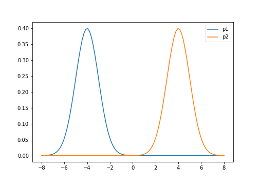
For example, let $p(x)$ be a mixture of two univariate Gaussians,
\[p(x) = \pi\mathcal{N}(\mu_1, \sigma^2_1) + (1-\pi)\mathcal{N}(\mu_2, \sigma^2_2)\]where $\pi$ controls the mixing proportions. Below is a plot of their densities where we set $\mu_1=-4, \mu_2=4$, and $\sigma^2_1=\sigma^2_2=1$.
Suppose we approximate $p(x)$ with a univariate Gaussian $q(x)$ by minimizing the KL divergence with respect to $q$’s variational parameters. We find that the KL divergence is lower when $q$ is centered around one of $p$’s modes, rather than spread between them. The figure below shows this for three possible orientations of $q$.
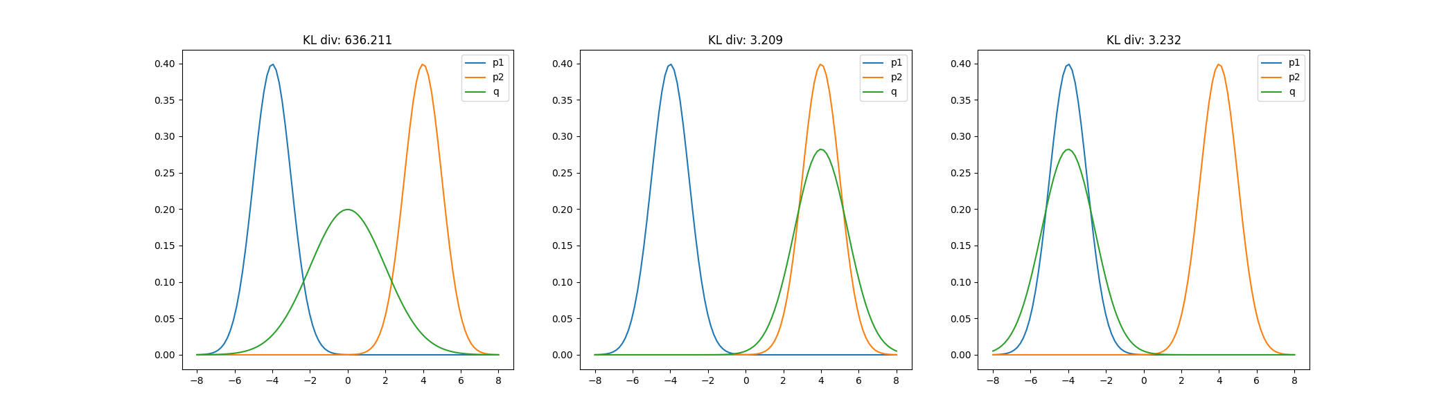
This mode-seeking behavior of the reverse KL divergence can be intuited from its form above. When $q$ is low but $p$ is high, then the divergence is low. However, if $q$ is high but $p$ is low, then the divergence is large.
Visualization
Next, we show a visualization of optimization using the reverse KL divergence. Consider data $x$ that is distributed according to a mixture of two-dimensional Gaussians,
\[p(x) = \pi \mathcal{N}_2(\mu_1, \Sigma_1) + (1-\pi) \mathcal{N}_2(\mu_2, \Sigma_2).\]This density is clearly multimodal, assuming $\mu_1 \neq \mu_2$.
Suppose we would like to approximate $p(x)$ with a single, unimodal Gaussian,
\[q(x) = \mathcal{N}(\lambda_{\mu}, \lambda_{\Sigma})\]where $\lambda_{\mu}$ is the variational mean, and $\lambda_{\Sigma}$ is the variational covariance.
Further, assume that we make a mean-field approximation, meaning that each dimension of the variational approximation is independent of the others. More concisely, we assume
\[\lambda_{\Sigma} = \text{diag}(\sigma^2_1, \sigma^2_2).\]In the experiment below, we assume the following:
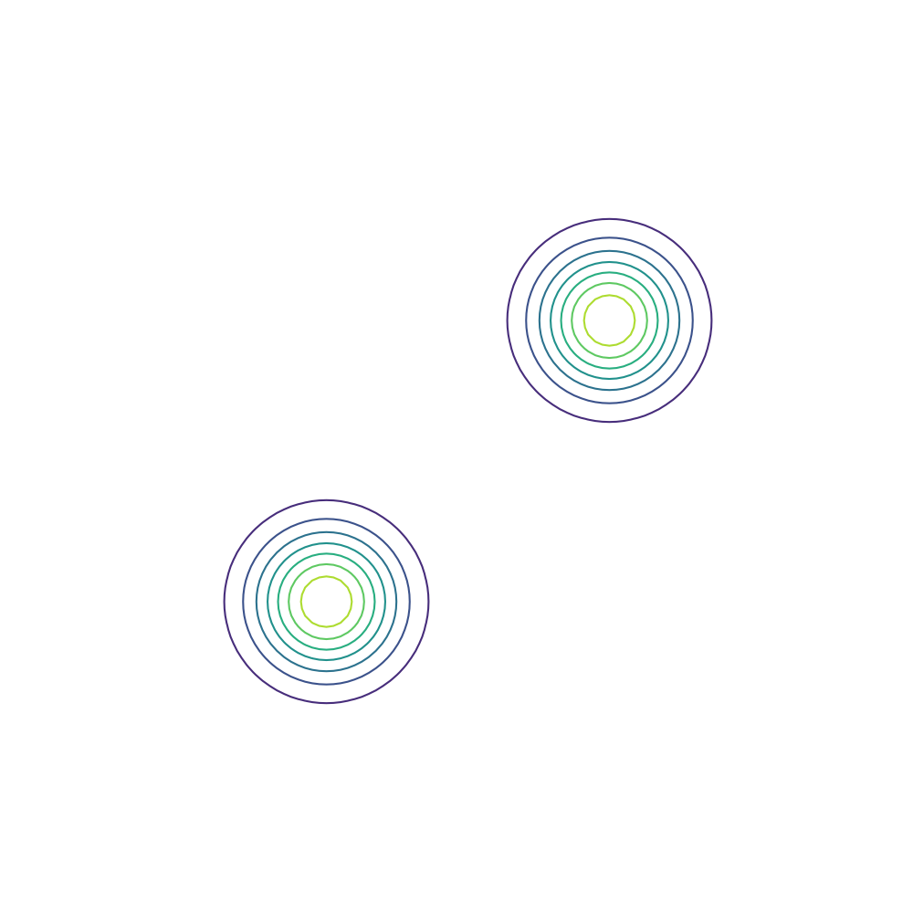
\[\mu_1 = \begin{bmatrix} -4 \\ -4 \end{bmatrix}, \mu_2 = \begin{bmatrix} 4 \\ 4 \end{bmatrix}, \Sigma_1 = \Sigma_2 = \begin{bmatrix} 1 & 0 \\ 0 & 1 \end{bmatrix}.\]Below is a contour plot of the density that we wish to approximate.
We optimize $\lambda_{\mu}, \lambda_{\Sigma}$ by minimizing the KL-qp divergence. In this post, we initialize the variational parameters as
\[\lambda_{\mu} =\begin{bmatrix} 0 \\ 0 \end{bmatrix}, \lambda_{\Sigma} = I_2.\]Below, we do this optimization using gradient descent and the Adam optimizer. We can visualize the optimization process by plotting the contours of the true density and the variational density over the iterations. The GIF below shows this visualization for our mixture of Gaussians example. The variational density is shown in the reddish colors.
As we can see, the variational density immediately moves to one of the modes (in this case, the mode with mean $\begin{bmatrix} 2 & 2 \end{bmatrix}^\top$).
Code
Below is the code for running the 2D Gaussian experiment above. It also creates the contour visualization. This is based on the examples in the autograd repo.
import matplotlib.pyplot as plt
from autograd import grad, value_and_grad
import autograd.numpy as np
from functools import partial
from autograd.scipy.stats import t, norm, multivariate_normal
from scipy.special import loggamma
from autograd.core import getval
from autograd.numpy import random as npr
from autograd.misc.optimizers import adam
from scipy.stats import multivariate_normal as mvn
from autograd.scipy.stats import multivariate_normal
import autograd.scipy.stats.t as t_dist

import matplotlib.animation as animation
import matplotlib.image as mpimg
import os

from autograd.scipy.special import logsumexp


class Model():

	def __init__(self, mean1, mean2, cov):

		self.mean1 = mean1
		self.mean2 = mean2
		self.cov = cov
		assert self.mean1.shape[0] == self.cov.shape[0]
		assert self.mean2.shape[0] == self.cov.shape[0]
		self.d = self.cov.shape[0]


	def log_density(self, zs):

		clust1_density = 0.5 * multivariate_normal.logpdf(zs, self.mean1, cov=self.cov)
		clust2_density = 0.5 * multivariate_normal.logpdf(zs, self.mean2, cov=self.cov)
		return np.logaddexp(clust1_density, clust2_density)

	def sample(self, n):
		num_clust1 = np.random.binomial(n=n, p=0.5)
		num_clust2 = n - num_clust1
		samples_mode1 = mvn.rvs(mean=self.mean1, cov=self.cov, size=num_clust1)
		samples_mode2 = mvn.rvs(mean=self.mean2, cov=self.cov, size=num_clust2)
		samples = np.vstack([samples_mode1, samples_mode2])
		return samples


class ApproxMFGaussian():

	def __init__(self):
		pass

	def log_density(self, var_param, z):
		# variational density evaluated at samples
		return multivariate_normal.logpdf(z, var_param[:2], np.diag(np.exp(var_param[2:] * 2)))

	def sample(self, var_param, S):
		stddevs = np.exp(var_param[2:])
		return var_param[:2] + seed.randn(S, 2) * np.expand_dims(stddevs, 0)

	def gradq(self, var_param, z):
		objective = lambda vparam : self.log_density(vparam, z)
		grad_q = grad(objective)
		return grad_q(var_param)

	def entropy(self, var_param):
		return 0.5 * 2 * (1.0 + np.log(2*np.pi)) + np.sum(var_param[2:] * 2)

d = 2

# Generate data
mean1 = np.array([-4, -4])
mean2 = np.array([4, 4])
cov = np.eye(d)

model = Model(mean1=mean1, mean2=mean2, cov=cov)
approx = ApproxMFGaussian()

S = 1000

# Variational parameters: first d elements are the mean, last d elements are the diagonal of log-covariance
variational_mean = np.array([0, 0])
variational_log_cov_diag = np.ones(d)
variational_param = np.concatenate([variational_mean, variational_log_cov_diag])


def objective(variational_param, iter):

	samples = approx.sample(variational_param, S)

	lik = np.mean(model.log_density(samples))
	entropy = approx.entropy(variational_param)
	elbo = lik + entropy

	return -elbo / S

seed = npr.RandomState(0)


def plot_isocontours(ax, func, xlimits=[-10, 10], ylimits=[-10, 10], numticks=101, cmap='viridis', label=''):
	x = np.linspace(*xlimits, num=numticks)
	y = np.linspace(*ylimits, num=numticks)
	X, Y = np.meshgrid(x, y)
	zs = func(np.concatenate([np.atleast_2d(X.ravel()), np.atleast_2d(Y.ravel())]).T)
	Z = zs.reshape(X.shape)
	plt.contour(X, Y, Z, cmap=cmap, label=label)
	ax.set_yticks([])
	ax.set_xticks([])

fig = plt.figure(figsize=(10, 10), facecolor='white')
ax = fig.add_subplot(111, frameon=False)
plt.ion()
plt.show(block=False)
target_distribution = lambda x : np.exp(model.log_density(x))
plot_isocontours(ax, target_distribution, label="p(z)")
plt.close()

fig = plt.figure(figsize=(10, 10), facecolor='white')
ax = fig.add_subplot(111, frameon=False)
plt.ion()
plt.show(block=False)

imgs = []
print("     Epoch     |    Objective     |    Param vals")
def print_perf(params, iter, grad):

	bound = objective(params, iter)
	message = "{:15}|{:20}|{:15}|{:15}{:15}|{:15}".format(iter, round(bound, 2), round(float(params[0]), 2), round(float(params[1]), 2), round(float(params[2]), 2), round(float(params[3]), 2))
	print(message)

	plt.cla()
	target_distribution = lambda x : np.exp(model.log_density(x))
	plot_isocontours(ax, target_distribution, label="p(z)")

	variational_contour = lambda x: mvn.pdf(x, params[:2], np.diag(np.exp(params[2:])))
	plot_isocontours(ax, variational_contour, cmap='plasma', label="q(z)")

num_epochs = 100
step_size = .1

optimized_params = adam(grad=grad(objective), x0=variational_param, step_size=step_size, num_iters=num_epochs, callback=print_perf)
References
- Duvenaud, David, and Ryan P. Adams. “Black-box stochastic variational inference in five lines of Python.” NIPS Workshop on Black-box Learning and Inference. 2015.
- Huggins, Jonathan, et al. “Validated variational inference via practical posterior error bounds.” International Conference on Artificial Intelligence and Statistics. PMLR, 2020.
- My code structure is largely based off of the code for viabel (i.e., the above paper).