Kernel PCA

$\DeclareMathOperator*{\argmin}{arg\,min}$ $\DeclareMathOperator*{\argmax}{arg\,max}$

Principal component analysis

Recall that PCA is a linear dimensionality reduction method that performs a change of basis in the data.

Given an $n \times p$ data matrix $\mathbf{X},$ PCA is performed using an eigendecomposition of the sample covariance matrix. Let $\mathbf{C} = n^{-1} \mathbf{X}^\top \mathbf{X}$ be the sample covariance matrix. Then the first $k$ principal components (where $k < p$) are given by the top $k$ eigenvectors of $\mathbf{C},$ which we denote as $\mathbf{U}_k = (\mathbf{u}_1, \cdots, \mathbf{u}_k).$ The columns of $\mathbf{U}$ can be interpreted as the directions in the data’s feature space with the highest variance.

Dimensionality reduction can then be performed by projecting the data onto these components:

\[\tilde{\mathbf{X}}_k = \mathbf{X} \mathbf{U}_k,\]

where $\tilde{\mathbf{X}}_k$ denotes the data matrix with reduced dimensionality.

Example

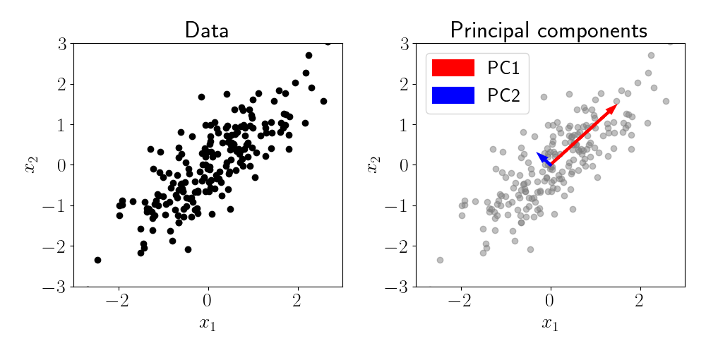
Consider a simple dataset with $p = 2$ features and $n = 200$ samples, where the two features are positively correlated with one another. This is demonstrated in the left panel of the figure below, where each black point represents a sample. We can clearly observe the correlation structure between the two features.

To verify that PCA can capture this correlation structure, we can fit PCA with $k=2$ and plot the resulting principal components. These are shown in the right panel of the figure below, where each PC is represented by a vector whose length is proportional to its respective eigenvalue. We can see that PC1 captures the main axis of correlation between the features, while PC2 captures the residual variation that is orthogonal to PC1.

**Left**: Data. **Right**: Principal components represented as vectors whose lengths are proportional to their respective eigenvalues.

Limitations of PCA

While PCA is useful for finding linear manifolds in a dataset, many data types contain nonlinear structure. As a simple motivating example, consider another two-dimensional dataset where there is a quadratic relationship between the features. The figure below shows this situation and the resulting principal components.

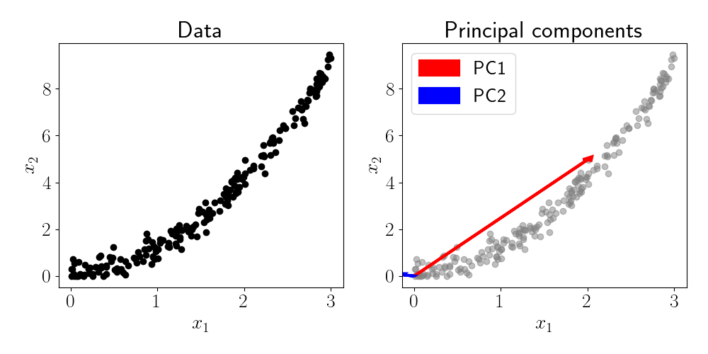
Although PC1 is generally pointing in the direction of highest variance, it does not fully capture the curved relationship between the two features. This is an inherent limitation of PCA: it is only equipped to identify linear relationships.

Kernel PCA

The linearity of PCA motivates the need to generalize this assumption to account for nonlinear structure in datasets. Kernel PCA, first proposed in 1997, is a natural extension of PCA that allows for identifying nonlinear structure.

While the theoretical underpinnings of kernel PCA are sophisticated, the basic idea is fairly simple: instead of operating in the native data space, we first perform a nonlinear transformation of the data, and then perform PCA in that space. This “nonlinear transformation” (more commonly called a basis expansion) can be chosen to reflect the analyst’s assumptions around what type of structure exists in the data.

We denote the function describing the basis expansion as $\phi : \mathbb{R}^p \rightarrow \mathbb{R}^q$ where in many cases $q > p.$ In words, $\phi$ transforms a data sample to a higher dimensional space. Common choices include the polynomial basis, which for $p=2$ is given by

\[\phi(\mathbf{x}) = (1, x_1, x_2, x_1 x_2, x_1^2, x_2^2).\]

We denote the matrix of basis-expanded data as

\[\Phi = (\phi(\mathbf{x}_1), \cdots, \phi(\mathbf{x}_n))^\top.\]

The hope is that in this transformed space, the data will exhibit linear structure so that PCA is now an appropriate choice. Given the covariance matrix $C = \Phi^\top \Phi,$ we can perform an eigendecomposition and obtain kernel-based PCs.

However, thanks to the kernel trick, we do not actually have to even expand the data with a function $\phi$. Since all we need to run PCA is the covariance matrix (rather than the basis-expanded data itself), the kernel trick allows us to directly compute the covariance matrix under a certain basis expansion through an equivalent kernel function $k(\cdot, \cdot).$ We can then compute the $ij$th element of the covariance matrix as $[C]_{ij} = k(\mathbf{x}_i, \mathbf{x}_j),$ and it will hold that $C = \Phi^\top \Phi$ for the appropriately chosen kernel function.

Example

Let’s return to our example from the figure above where the two features of the data have a nonlinear relationship. Here, for visualization we’ll demonstrate an application of kernel PCA to this dataset using a basis function approach, rather than leveraging the kernel trick.

Suppose we choose the basis function $\phi(\mathbf{x}) = [x_1, \sqrt{x_2}].$ The data and its transformed version are shown in the figure below.

We can see that after applying the basis function, the two features appear to have a linear relationship. It now seems appropriate to fit PCA.

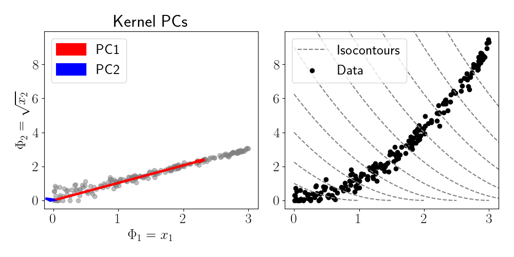
The left panel of the figure above shows the two PCs of the transformed data. We can see that PC1 accounts for the majority of the variance in the data. We can also visualize the regions of the data space that are identified to have similar features values. While in traditional PCA, these “isocontours” would be straight lines or hyperplanes across the space, we see that kernel PCA identifies nonlinear regions of the space that have equal feature value.

References

Schölkopf, Bernhard, Alexander Smola, and Klaus-Robert Müller. “Kernel principal component analysis.” International conference on artificial neural networks. Springer, Berlin, Heidelberg, 1997.