Andy Jones
Just-in-time compilation and JAX
Most research in machine learning and computational statistics focuses on advancing methodology. However, a less-hyped topic — but an extremely important one — is the actual implementation of these methods using programming languages and compilers. Here, we explore one recent application of ideas from compilers to machine learning: just-in-time (JIT) compilation for machine learning libraries. Specifically, we’ll show how JAX implements a JIT option and the advantages of using it.
Compiled vs. interpreted languages
To understand the advantage of JIT compilation, we first have to understand the difference between compiled and interpreted languages. Note that the distinction between these two is less black-and-white than I say below, as many hybrids exist today.
Roughly, a compiled language translates the entire program to machine code prior to running the code. This compilation step typically finds certain optimizations to make the code faster. When the code is actually executed, it uses this optimized machine code to run the original source code. Perhaps the most famous compiled languages are C and C++. This two-step process (compile then execute) is evident from the way we work with C code. Consider Hello, World! in C:
#include <stdio.h>
int main() {
   printf("Hello, World!");
}
We first have to compile this program with gcc on the command line.
gcc helloworld.c -o helloworld
We can then run the program by calling the resulting binary executable:
./helloworld
On the other hand, interpreted languages execute the source code instruction-by-instruction, avoiding translating the entire source code to machine code. Instead, it uses an “interpreter” that identifies each function call and calls the relevant machine code function on the fly. One of the most widely-used interpreted languages (especially in the machine learning world) is Python. Hello, World! in Python is just one line (print("Hello, World!")), which can be executed with just one command line call: python helloworld.py. Notice that there’s no required compilation step.
While the tradeoffs between compiled and interpreted languages can be complicated (and even this distinction is a bit misleading in some cases), we can roughly think of the difference as follows.
- Compiled languages are fast to execute, but it’s difficult to write efficient compilers, which can make compiled languages cumbersome.
- Interpreted languages are easier to write and more flexible in some situations, but are slower to execute.
Just-in-time compilation
In the middle between interpretation and compilation, we have just-in-time (JIT) compilation. We can think of JIT compilation as a hybrid of the two paradigms discussed above.
Rather than compiling the entire program prior to execution, a JIT approach compiles the code function-by-function as needed. Said a different way, a JIT compiler compiles a piece of code only right before you need it at run time, hence the name “just-in-time”.
The advantage of JIT compilation is that we get the speedups from compilation along with the flexibility of interpretation. Instead of “caching” the entire program as machine code, we can cache smaller code snippets, which we can reuse every time we need to run the same snippet.
While JIT compilation is a well-established idea in the fields of programming languages and compilers, its application in machine learning and scientific computing hasn’t occurred until recently. One framework that has popularized JIT compilation recently is JAX, which we’ll explore next.
JAX
Python dominates most of the machine learning world as the language of choice. The fact that Python is an interpreted language begs the question whether we can make make it more performant for ML systems by incorporating ideas from compiled languages.
JAX is a programming framework for scientific computing and machine learning that tries to bridge this divide. There are several different functionalities to JAX, but the most unique one is its JIT compiler. This form of program execution can speed up machine learning programs with just one extra function calls.
To see how it works, let’s see a simple example. Consider the following function that adds two numbers.
import jax.numpy as np
def add(a, b):
	return np.add(a, b)
If we call this function as-is, we’ll rely on the Python interpreter to route each call to the appropriate add function. However, we can translate this function into a compiled function using jax.jit as follows:
import jax
add_jitted = jax.jit(add)
If we examine the type of add_jitted, we’ll find that it’s of the type <class 'jaxlib.xla_extension.jax_jit.CompiledFunction'>. In other words, this function is now compiled using the XLA compiler, which is specifically designed for linear algebra and matrix computation. Now, whenever we call add_jitted, we’ll directly use the compiled version, rather than using Python’s interpreter.
Let’s test how much faster the jitted function is in this case. Here’s a short code snipped to compare the run-time of add and add_jitted.
n_repeats = 5
n_range = [10, 100, 500, 1000, 5000, 10000]
nojit_times = onp.zeros((n_repeats, len(n_range)))
jit_times = onp.zeros((n_repeats, len(n_range)))

for ii, n in enumerate(range(n_repeats)):
	for jj, n in enumerate(n_range):

		# JIT
		start_time = time.time()
		[add_jitted() for _ in range(n)]
		end_time = time.time()

		jit_times[ii, jj] = end_time - start_time

		# No JIT
		start_time = time.time()
		[add() for _ in range(n)]
		end_time = time.time()

		nojit_times[ii, jj] = end_time - start_time
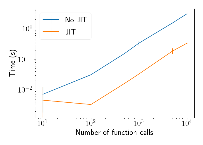
Plotting the time across different numbers of calls, we see that add_jitted is a constant amount of time faster than add. This is expected because each function call will be a constant time faster, so repeating that call multiple times will still yield a constant margin between the two functions.
Not that, while this example used simple addition of two scalars, XLA and JAX are especially optimized for more complicated linear algebra computation. In particular, they’re optimized for computation graphs, matrix multiplication, and gradient computation.
Other functionalities of JAX
While this post focuses on the JIT compiler aspect of JAX, we can really think of it as a more general framework for computational models in Python. It also allows for automatic differentiation, function vectorization, and parallelization.