Andy Jones
James-Stein estimator
The James-Stein estimator dominates the MLE by sharing information across seemingly unrelated variables.
Admissibility
Suppose we want to estimate a parameter (or parameter vector) $\theta$ in some statistical model. Broadly, we do this by constructing an “estimator” $\theta(x)$, which is a function of the data $x$. Let $\theta^\star$ denote the true value of $\theta$ (the one that actually corresponds to the data generating process).
Given a set of data observations $x$, we can assess the quality of the estimator using a loss function $\mathcal{L}(\theta^\star, \hat{\theta})$, which compares the true $\theta^\star$ to our estimate. Lower loss values typically correspond a “better” estimator. Example loss functions are the squared (L2) error $\mathcal{L}(\theta^\star, \hat{\theta}) = ||\theta - \theta^\star||_2^2$ and the L1 error $\mathcal{L}(\theta^\star, \hat{\theta}) = ||\theta - \theta^\star||_1$.
If we want to assess the estimator over all possible data (not just one set of observations), we can compute the estimator’s risk, which is the expectation of $\mathcal{L}$ over the data distribution $p(x | \theta^\star)$.
Specifically, given a loss function $\mathcal{L}$, the risk function is defined as
\[R(\theta^\star, \hat{\theta}) = \mathbb{E}_{p(x | \theta^\star)}[\mathcal{L}(\theta^\star, \hat{\theta}(x))].\]Now, we can use the risk function to compare different estimators. Suppose we have two different estimators $\hat{\theta}^{(1)}$ and $\hat{\theta}^{(2)}$. For any true parameter value $\theta^\star$, we can then compute the risk of each, $R(\theta^\star, \hat{\theta}^{(1)})$ and $R(\theta^\star, \hat{\theta}^{(2)})$, and compare them.
Often, one estimator will have a lower risk for some values of $\theta^\star$ and a higher risk for others. However, we say that an estimator $\hat{\theta}^{(1)}$ dominates another estimator $\hat{\theta}^{(2)}$ if $\hat{\theta}^{(1)}$ doesn’t has a higher risk for any $\theta^\star$ and has a lower risk for at least one value of $\theta^\star$. In other words, $\hat{\theta}^{(1)}$ dominates another estimator $\hat{\theta}^{(2)}$ if:
- $R(\theta^\star, \hat{\theta}^{(1)}) \leq R(\theta^\star, \hat{\theta}^{(2)}) \;\;\; \forall \theta^\star \in \Theta.$
- $\exists \theta^\star \text{ such that } R(\theta^\star, \hat{\theta}^{(1)}) < R(\theta^\star, \hat{\theta}^{(2)})$
Finally, an estimator is admissible if it’s not dominated by any other estimator. Otherwise, we say it’s inadmissible.
Stein phenomenon
Consider $p$ Gaussian random variables $X_1, \dots, X_p$, where
\[X_i \sim \mathcal{N}(\mu_i, \sigma^2), \;\;\; i = 1, \dots, p\]where $\sigma^2$ is known, and we’d like to estimate each $\mu_i$.
Suppose our data consists of one observation of each variable $x_1, \dots, x_p$. With such little information to work with, under the squared error loss, the least squares estimator (maximum likelihood estimator AKA “ordinary” estimator AKA “usual” estimator) would simply estimate each mean as the data point’s value:
\[\hat{\mu_i}^{(LS)} = x_i.\]However, Charles Stein discovered interesting and surprising result:
The least squares estimator is inadmissible with respect to the squared error loss when $p \geq 3$. In other words, the least squares estimator is dominated by another estimator.
Prof. John Carlos Baez summarizes this unintuitive result nicely in this Twitter thread:
I have a Gaussian distribution like this in 2d. You know its variance is 1 but don't know its mean. I randomly pick a point (x₁,x₂) according to this distribution and tell you. You try to guess the mean.
— John Carlos Baez (@johncarlosbaez) August 25, 2020
Your best guess is (x₁,x₂).
But this is not true in 3d!!!
(1/n) pic.twitter.com/pWPD8sFmZ6
So, what’s this other estimator?
James-Stein estimator
The James-Stein estimator (concocted by Charles Stein and Willard James) is
\[\hat{\mu}_i^{(JS)} = \left( 1 - \frac{(p - 2) \sigma^2}{||\mathbf{x}||_2^2} \right) x_i.\]where $\mathbf{x}$ is the $p$-vector of observations.
Notice that this estimator is essentially multiplying each $x_i$ by a term $\left( 1 - \frac{(p - 2) \sigma^2}{||\mathbf{x}||_2^2} \right)$ that depends on the other variables as well.
To start building intuition about what this estimator is doing, consider the case when $p = 3$, and $\sigma^2 = 1$. Then the James-Stein estimator reduces to
\[\hat{\mu}_i^{(JS)} = \left( 1 - \frac{1}{||\mathbf{x}||_2^2} \right) x_i.\]Since $||\mathbf{x}||_2^2 \geq 0$, we know that $\left( 1 - \frac{1}{||\mathbf{x}||_2^2} \right) < 1$. If $||\mathbf{x}||_2^2 > 1$, then the estimator shrinks $\mu_i$ toward 0 compared to the least squares estimator. If $||\mathbf{x}||_2^2 < 1$, the estimator adjusts the LS estimator even further, and even performs a sign flip.
More generally, if $||\mathbf{x}||_2^2 > (p - 2) \sigma^2$, then the James-Stein estimator shrinks each $\mu_i$ toward zero. In other words, if the overall (L2) magnitude of the data vector $\mathbf{x}$ exceeds the variance (multiplied by $p-2$), the James-Stein estimator “regularizes” the estimates $\mu_i$ by shrinking it toward zero.
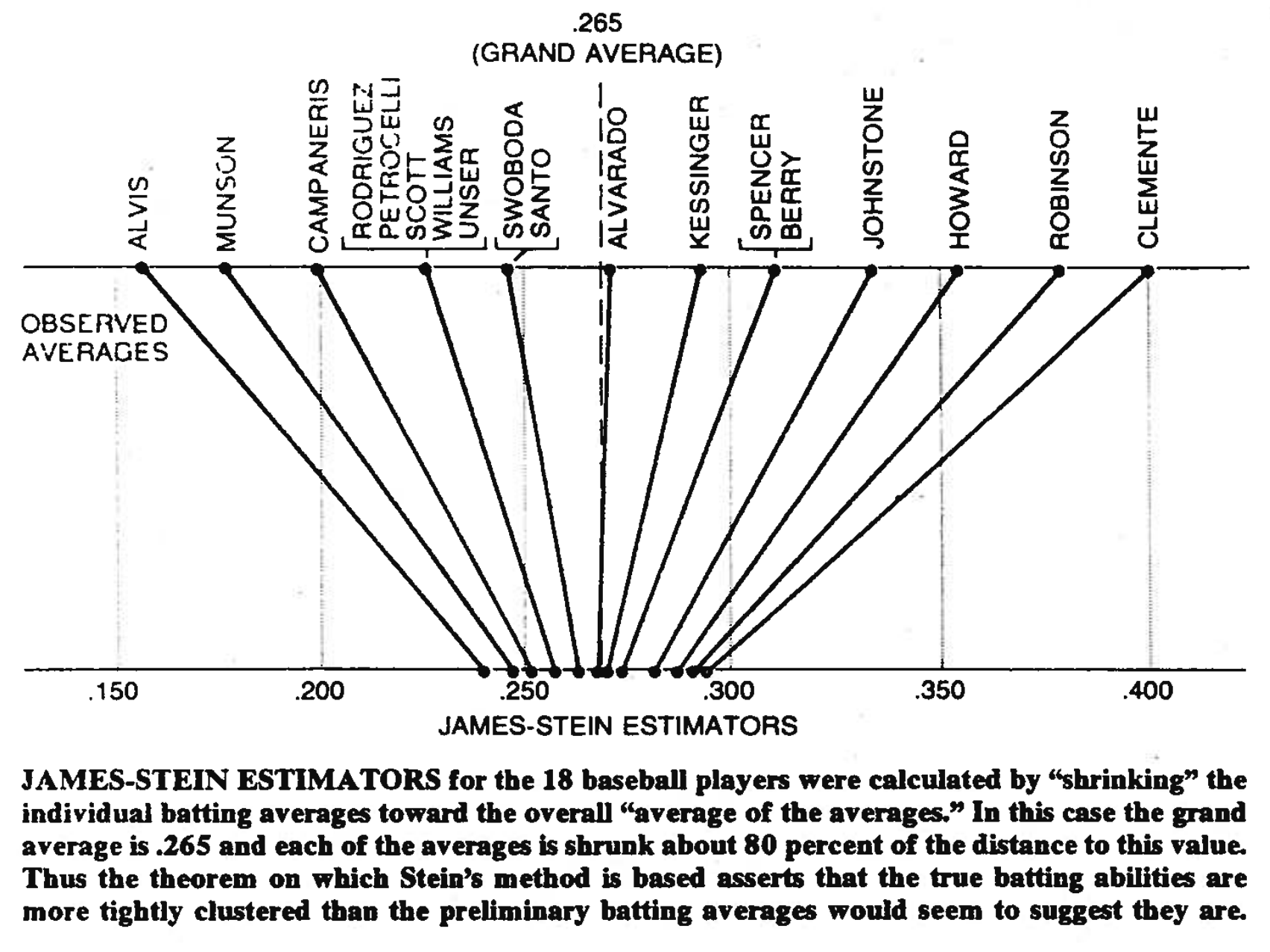
Another way to think about the James-Stein estimator is as a “shrinkage” estimator. The James-Stein estimator has the effect of nudging each individual $\hat{\mu}_i$ toward the overall average of the data points, $\bar{\mathbf{x}} = \frac1n \sum\limits_{i=1}^n x_i$. Brad Efron and Carl Morris have a nice figure demonstrating this in their paper “Stein’s Paradox in Statistics”. In the figure below, the top row shows the batting averages for 18 baseball players, and the bottom row shows the corresponding James-Stein estimator of each. Notice how the estimates move closer together, thereby sharing information across them.
Relationship to empirical Bayes
The James-Stein estimator also has strong connections to the empirical Bayes methodology. Under an empirical Bayes framework, instead of completely marginalizing out the prior (as in a fully Bayesian treatment), we estimate the prior from the data.
For example, consider again $p$ Gaussian random variables $X_1, \dots, X_p$, where
\[X_i \sim \mathcal{N}(\mu_i, \sigma^2), \;\;\; i = 1, \dots, p\]where $\sigma^2$ is known, and we’d like to estimate each $\mu_i$. Now, let’s place a shared normal prior on each $\mu_i$:
\[\mu_i \sim \mathcal{N}(0, \tau^2), \;\;\; i = 1, \dots, p.\]We could manually set $\tau^2$ to some value, e.g. $\tau^2 = 1$, or we could place another prior on it and integrate it out.
On the other hand, the empirical Bayes approach seeks to estimate $\tau^2$ from the data itself, leveraging information across observations.
First, notice that the posterior $p(\mu_i | X)$ is
\[p(\mu_i | X_i) = \frac{p(X_i | \mu_i) p(\mu_i)}{\int p(X_i | \mu_i) p(\mu_i) d\mu_i)}.\]After some arithmetic and extra work to solve the integral (e.g., through completing the square), we see that the posterior is also Gaussian:
\[\mu_i | X_i \sim \mathcal{N}\left(\frac{\tau^2}{\tau^2 + \sigma^2} X_i, \frac{\tau^2}{\tau^2 + \sigma^2} \right).\]So the “Bayes” estimator (if we just take the expectation of the posterior above) is
\[\hat{\mu}_i^{(\text{Bayes})} = \frac{\tau^2}{\tau^2 + \sigma^2} X_i.\]Notice that this estimator is effectively shrinking $X_i$ toward zero.
Now, what if we want a more principled way to set $\tau^2$ above, as opposed to just setting it to some value manually? One way to do this would be to look for an unbiased estimator $\hat{\alpha}$ of the “shrinkage coefficient” $\frac{\tau^2}{\tau^2 + \sigma^2}$ such that
\[\mathbb{E}_{p(X_i)}[\hat{\alpha}] = \frac{\tau^2}{\tau^2 + \sigma^2}.\]Notice that the marginal distribution
\[p(X_i) = \int p(X_i | \mu_i) p(\mu_i) d\mu_i\]is again Gaussian with
\[X_i \sim \mathcal{N}(0, \sigma^2 + \tau^2).\]Recall that for a Guassian random vector $\mathbf{z} = (z_1, \dots, z_p)^\top$, its squared L2-norm $||\mathbf{z}||_2^2$ will follow a $\chi^2$ distribution with $p$ degrees of freedom. Furthermore, $1 / ||\mathbf{z}||_2^2$ will follow an inverse-$\chi^2$ distribution, again with $p$ degrees of freedom.
In the case of our data, we can notice that the vector of data $\mathbf{X} = (X_1, \dots, X_p)^\top$ has a norm $||\mathbf{X}||_2^2$ that follows a scaled $\chi^2$ (scaled by $\sigma^2 + \tau^2$). Consequently,
\[\frac{1}{||\mathbf{X}||_2^2} \sim \frac{1}{\tau^2 + \sigma^2} \cdot \text{inverse-}\chi^2_p.\]Notice that the expectation of the James-Stein estimator’s coefficient (let’s call it $\hat{\alpha}^{(JS)}$) is unbiased in this case!
\begin{align} \mathbb{E}[\hat{\alpha}^{(JS)}] &= \mathbb{E}\left[\left( 1 - \frac{(p - 2) \sigma^2}{||\mathbf{X}||_2^2} \right)\right] \\ &= 1 - \mathbb{E}\left[\left(\frac{(p - 2) \sigma^2}{||\mathbf{X}||_2^2} \right)\right] \\ &= 1 - (p - 2) \sigma^2 \mathbb{E}\left[\frac{1}{||\mathbf{X}||_2^2} \right] \\ &= 1 - (p - 2) \sigma^2 \frac{1}{(\tau^2 + \sigma^2) (p - 2)} \\ &= 1 - \frac{\sigma^2}{\tau^2 + \sigma^2} \\ &= \frac{\tau^2}{\tau^2 + \sigma^2} \\ \end{align}
Thus, although Charles Stein didn’t originally derive the James-Stein estimator this way, we see that it also arises as a particular case of performing empirical Bayes.
References
- Stein, Charles. “Inadmissibility of the usual estimator for the mean of a multivariate distribution.” Proc. Third Berkeley Symp. Math. Statist. Prob. Vol. 1. 1956.
- Wikipedia entry on admissibility
- Wikipedia entry on the James-Stein estimator
- Efron, Bradley, and Carl Morris. “Stein’s paradox in statistics.” Scientific American 236.5 (1977): 119-127.
- Professor Efron’s notes on the James-Stein estimator.
- This StackOverflow post
- Blog post by Austin Rochford on the relationship between empirical Bayes and the James-Stein estimator.