Inducing points for Gaussian Processes

Inducing points provide a strategy for lowering the computational cost of Gaussian process prediction by closely modeling only a subset of the input space.

Computing the posterior predictive distribution for Gaussian processes is computationally expensive — typically $O(n^3)$ where $n$ is the number of data points. Inducing points lower this computation cost by selecting a few points in the input space to treat as “landmarks” for prediction.

Gaussian process regression

Recall that a Gaussian process is a collection of random variables $Y_1, Y_2, \dots$ such that any finite subset of these random variables follows a multivariate normal distribution. In particular,

where ${i_1, \dots, i_n}$ is an arbitrary set of indices.

Gaussian processes are commonly used to model regression functions. Given a set of response variables $Y_1, \dots, Y_n$, we can model their density as a multivariate normal whose covariance is a function of a set of corresponding input variables $X_1, \dots, X_n$. Specifically,

Here, $K(X, X)$ denotes a kernel function $k$ applied to the inputs,

where $k(x, x^\prime)$ is a Mercer kernel.

Another common (and equivalent) form of this model is to write it in terms of a Gaussian process prior over an arbitrary regression function $f$,

Note that the functional form is completely determined by the choice of kernel function (and the mean function, although we’ve set it to $0$ for simplicity here).

A very attractive property of Gaussian processes is that we can exploit the nice properties of the multivariate normal distribution to get closed-form expressions for predictive and posterior distributions. To see this, suppose we have $t$ test points $X_1^\star, \dots, X_t^\star$. We can get a closed-form expression for the predictive distribution:

where

\begin{align} \mu &= K_{X^\star X} (K_{XX} + \sigma^2 I_n)^{-1} Y \\ \Sigma &= K_{X^\star X} (K_{XX} + \sigma^2 I_n)^{-1} K_{XX^\star} + \sigma^2 I_t). \end{align}

Notice that the computation time for computing this predictive distribution is dominated by the inversion of the $n\times n$ matrix $K_{XX} + \sigma^2 I_n$. This operation will cost $O(n^3)$ in general.

Inducing points

Inducing points are essentially motivated by the following question: Rather than modeling the entire set of inputs $X$, what if we instead focused on modeling a smaller subset of regions of the input space? If we were able to do this, we could exploit any redundancy and correlation in the input space to reduce computation time.

To do this, we first have to choose a set of inducing points, which are a sort of “imaginary” data points. Let’s call the $m$ inducing points $\bar{x}_1, \dots, \bar{x}_m$ and their corresponding imaginary outputs $\bar{f}_1, \dots, \bar{f}_m$. We use the $f$ notation for the outputs because we assume they’re noiseless observations from the Gaussian process (we can do this because they’re imaginary).

Of course, we can write down the predictive distribution for these inducing points using the equations above, $p(\bar{f} | \bar{X}, X, Y)$. The key idea is then that we assume that these inducing points and responses completely explain any new predictions, and these predictions are no longer directly dependent on the data $(X, Y)$. In particular, we assume

We can then integrate the inducing point outputs $\bar{f}$ in closed form:

This turns out to be another Gaussian,

\begin{align} Y^\star_j | X^\star_j, X, Y, \bar{X} &\sim \mathcal{N}(\widehat{\mu}, \widehat{\sigma^2}) \\ \widehat{\mu} &= K_{X^\star \bar{X}} Q_m^{-1} K_{\bar{X} X} (\Lambda + \sigma^2 I_n)^{-1} Y \\ \widehat{\sigma^2} &= K_{X^\star X^\star} - K_{X^\star \bar{X}} (K_{\bar{X}\bar{X}}^{-1} - Q_m^{-1}) K_{\bar{X} X^\star} + \sigma^2 \\ Q_m &= K_{\bar{X} \bar{X}} + K_{\bar{X} X} (\Lambda + \sigma^2 I_n)^{-1} K_{X \bar{X}} \\ \Lambda &= \text{diag}(\lambda) \\ \lambda_i &= k(X_i, X_i) - K_{X_i \bar{X}} K_{\bar{X}\bar{X}}^{-1} K_{\bar{X}X_i}. \end{align}

Now we can analyze the computational cost of computing this predictive distribution. Notice that matrix inversion is no longer the bottleneck: inverting the diagonal matrix $\Lambda + \sigma^2 I_n$ will only cost $O(n)$. Rather, matrix multiplication will be the main source of any slow-down — in particular, the product of an $m \times n$ matrix with an $n \times m$ matrix. This will cost $O(m^2 n)$. If $m<n$ (which we always assume, given that our initial goal was to focus on a small subset of the input space), then we immediately have a speedup compared to full GP regression, which cost $O(n^3)$.

Of course, there is a price to be paid in accuracy. Since we’re only choosing a small set of inducing points, any predictions we make will be worse than our predictions using the full data set. Choosing “good” inducing points — ones that are representative of the dataset — is then the name of the game. One option is to optimize the locations of the inducing points by maximizing the marginal likelihood.

Below, we show some simple examples in which we select the inducing points a priori, and show the resulting predictions.

Experiments

GP regression with inducing points

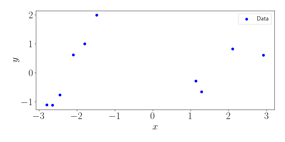
Let’s try a simple experiment to visualize how inducing points work. To start, let’s sample some data from a GP regression model with an exponentiated quadratic kernel. This kernel’s form is given by

where $\ell$ is the length scale. We will take $\ell=1$ for all experiments here. Notice that this kernel is essentially measuring the density of a Gaussian with mean $x^\prime$ at point $x$ (or vice versa). Our $n=10$ sampled data points look like this:

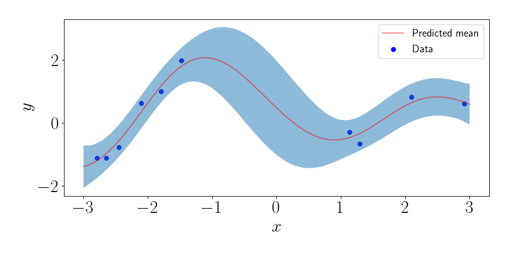
Using the full GP regression predictive distribution, we can compute dense predictions along the $x$ axis. This gives us a measure of uncertainty. Below, we plot the predicted mean, as well as two times the standard deviation of each marginal predictive distribution.

Now, let’s choose a set of inducing points. Here, I uniformly sample $m=2$ inducing points. The vertical lines represent their locations. Again, we can plot the predictions based on the inducing point method.

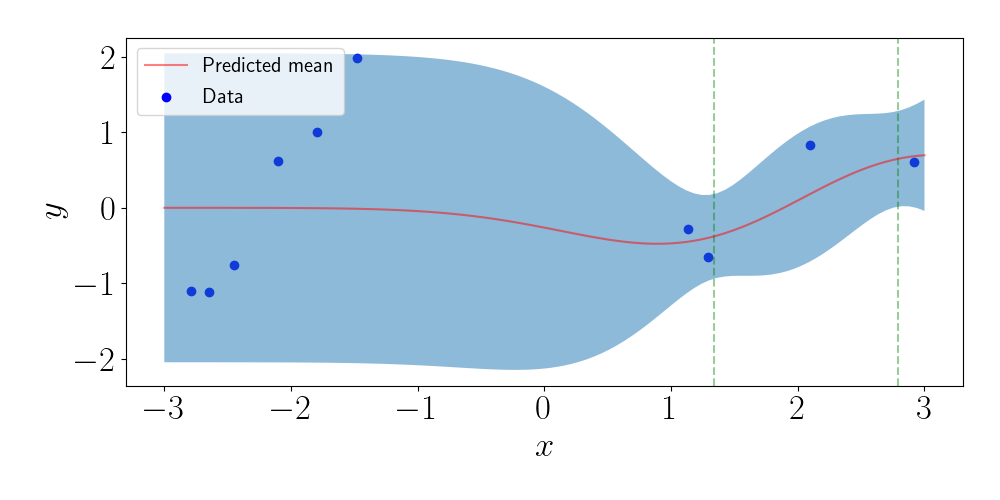
We can see that the predictions near the inducing points resemble those for the full GP. However, as we move away from the inducing points, the predictions revert to the prior, even though we have data in those regions.

Closer look with just one data point

To see the effect of the location of the inducing points more closely, consider the case when we have just one data point. Using the same kernel as above, our full GP predictions look like this:

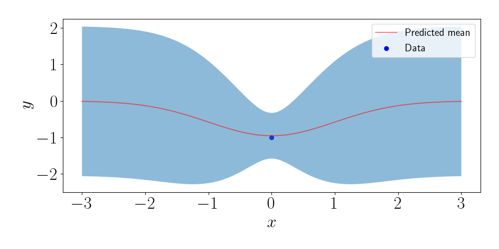
Now, let’s use just one inducing point. (Of course, this doesn’t make much sense practically when $n=1$, but we’re just working for the sake of understanding right now). In the figure below, we show the predictive values for four different values of the inducing point.

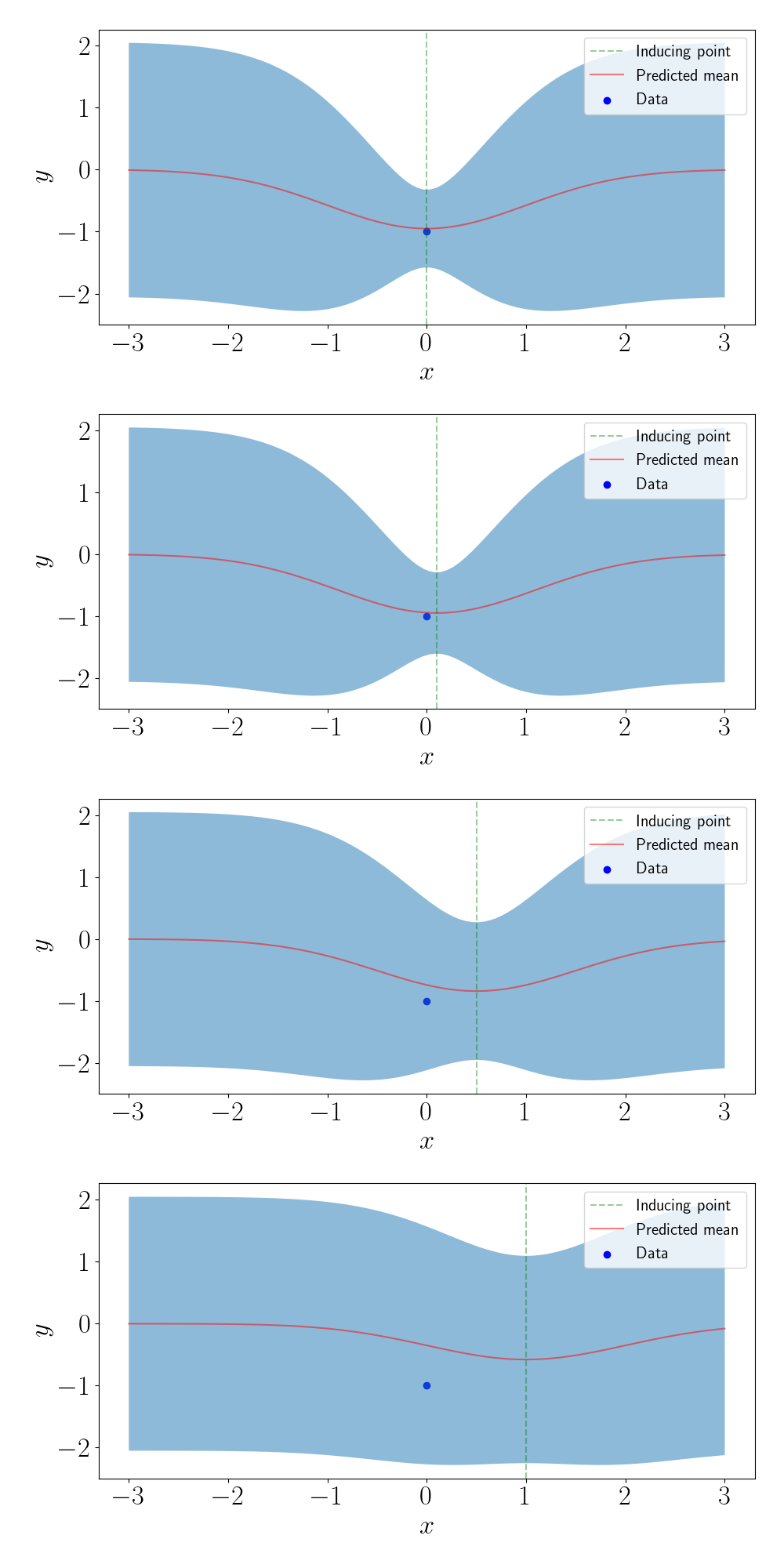
We can see that, as the inducing point moves farther away from the data point, the predictions get closer and closer to the prior.

Code

import numpy as np
import matplotlib.pyplot as plt
import seaborn as sns
from sklearn.gaussian_process.kernels import RBF
from scipy.stats import multivariate_normal as mvn
import matplotlib
inv = np.linalg.inv


font = {"size": 25}
matplotlib.rc("font", **font)
matplotlib.rcParams["text.usetex"] = True

# Set up kernel
k = RBF()

# Draw samples from GP
n = 10
sigma2 = .05
x = np.random.uniform(low=-3, high=3, size=n)
Kxx = k(np.expand_dims(x, 1), np.expand_dims(x, 1))
y = mvn.rvs(mean=np.zeros(n), cov=Kxx + sigma2 * np.eye(n))

plt.figure(figsize=(10, 5))
plt.scatter(x, y, c="blue", label="Data")
plt.xlabel(r"$x$")
plt.ylabel(r"$y$")
plt.legend(prop={'size': 15})
plt.tight_layout()
plt.savefig("./out/inducing_points_data.png")
plt.close()

# Get predictions from GP
n_test = 100
xstar = np.linspace(-3, 3, n_test)
Kxstarx = k(np.expand_dims(xstar, 1), np.expand_dims(x, 1))
Kxstarxstar = k(np.expand_dims(xstar, 1), np.expand_dims(xstar, 1))
ystar_mean = Kxstarx @ inv(Kxx + sigma2 * np.eye(n)) @ y
ystar_cov = Kxstarxstar - Kxstarx @ inv(Kxx + sigma2 * np.eye(n)) @ Kxstarx.T + sigma2
band_width = 2 * np.sqrt(np.diag(ystar_cov))
lower = ystar_mean - band_width
upper = ystar_mean + band_width

plt.figure(figsize=(10, 5))
plt.scatter(x, y, c="blue", label="Data")
plt.plot(xstar, ystar_mean, c="red", alpha=0.5, label="Predicted mean")
plt.fill_between(xstar, lower, upper, alpha=0.5)
plt.xlabel(r"$x$")
plt.ylabel(r"$y$")
plt.legend(prop={'size': 15})
plt.tight_layout()
plt.savefig("./out/inducing_points_gp_predictions.png")
plt.close()


# Create inducing points
m = 2
xbar = np.random.uniform(low=-3, high=3, size=m)

# Get predictions using inducing points
Kxbarxbar = k(np.expand_dims(xbar, 1), np.expand_dims(xbar, 1))
Kxbarx = k(np.expand_dims(xbar, 1), np.expand_dims(x, 1))
Kxstarxbar = k(np.expand_dims(xstar, 1), np.expand_dims(xbar, 1))
Lambda = np.zeros(n) #np.diag(np.diag(Kxx) - np.diag(Kxbarx.T @ inv(Kxbarxbar) @ Kxbarx))
for ii in range(n):
  Lambda[ii] = Kxx[ii, ii] - Kxbarx.T[ii, :] @ inv(Kxbarxbar) @ Kxbarx[:, ii]
Lambda = np.diag(Lambda)
assert np.all(Lambda >= 0)
Qm = Kxbarxbar + Kxbarx @ inv(Lambda + sigma2 * np.eye(n)) @ Kxbarx.T
ystar_mean = np.zeros(n_test)
ystar_vars = np.zeros(n_test)
for ii in range(n_test):
  ystar_mean[ii] = Kxstarxbar[ii, :] @ inv(Qm) @ Kxbarx @ inv(Lambda + sigma2 * np.eye(n)) @ y
  ystar_vars[ii] = Kxstarxstar[ii, ii] - Kxstarxbar[ii, :] @ (inv(Kxbarxbar) - inv(Qm)) @ Kxstarxbar.T[:, ii] + sigma2




band_width = 2 * np.sqrt(ystar_vars)
lower = ystar_mean - band_width
upper = ystar_mean + band_width

plt.figure(figsize=(10, 5))
plt.scatter(x, y, c="blue", label="Data")
for ii in range(m):
  plt.axvline(xbar[ii], alpha=0.4, linestyle="--", c="green")
plt.plot(xstar, ystar_mean, c="red", alpha=0.5, label="Predicted mean")
plt.fill_between(xstar, lower, upper, alpha=0.5)
plt.xlabel(r"$x$")
plt.ylabel(r"$y$")
plt.legend(prop={'size': 15})
plt.tight_layout()
plt.savefig("./out/inducing_points_ip_predictions.png")
plt.close()

References

• Snelson, Edward, and Zoubin Ghahramani. “Sparse Gaussian processes using pseudo-inputs.” Advances in neural information processing systems 18 (2005): 1257-1264.