Hamiltonian Monte Carlo

Hamiltonian Monte Carlo (HMC) is an MCMC method that borrows ideas from physics. Here, we’ll give a brief overview and a simple example implementation.

Introduction

Consider the setting of Bayesian inference, in which we’re interested in describing the posterior distribution of some parameters $\boldsymbol{\theta}$ given some data $X$: $p(\boldsymbol{\theta} | X)$. At a very general level, MCMC algorithms attempt to explore the parameter space such that the distribution over states is representative of the posterior distribution. This requires a systematic way to decide how to move from point to point in the parameter space. In particular, given a (typically random) starting point $\boldsymbol{\theta}_0$, we’d like to visit a sequence of states $\boldsymbol{\theta}_1, \boldsymbol{\theta}_2, \dots$ so that eventually their distribution approximates the posterior. Various MCMC algorithms have unique ways of “proposing” the next step $\boldsymbol{\theta}_{t+1}$, given the current state $\boldsymbol{\theta}_{t}$ – see this previous post for a brief review.

Hamiltonian Monte Carlo

Hamiltonian Monte Carlo (HMC) is a Markov Chain Monte Carlo (MCMC) algorithm that can make mixing much more efficient compared to other MCMC algorithms, like Gibbs Sampling and Metropolis-Hastings procedures. HMC is built on the idea of modeling movement in the chain’s state space as a physical system.

Specifically, HMC decides on the sequence of steps by treating the parameters as the location of a “particle” on a curved landscape. Given the current position and momentum of the particle and the gradient of the landscape, HMC pushes the particle through the landscape by simulating its motion using well-established physics principles.

The “landscape” is defined by the log joint probability of the parameters

In order to initially get the particle moving, we must supply the momentum of the particle, $\boldsymbol{r}$ (which is a $p$-vector), at the start of each iteration. Suppose we draw the momentum from a spherical Gaussian:

Then, the joint density of the parameters and the momentum is given by

\begin{align} p(\boldsymbol{\theta}, \boldsymbol{r}) &= \exp(\mathcal{L}(\boldsymbol{\theta})) 2\pi^{-p/2} \exp\left( -\frac12 \boldsymbol{r}^\top \boldsymbol{r} \right) \\ &\propto \exp(\mathcal{L}(\boldsymbol{\theta})) \exp\left( -\frac12 \boldsymbol{r}^\top \boldsymbol{r} \right) \\ &\propto \exp\left(\mathcal{L}(\boldsymbol{\theta}) -\frac12 \boldsymbol{r}^\top \boldsymbol{r} \right). \\ \end{align}

Conveniently, we can interpret this joint density in terms of physical principles. We’ve already mentioned that $\boldsymbol{\theta}$ is the particle’s position and $\boldsymbol{r}$ is its momentum. Now, we can add a couple other interpretations.

First, we can interpret $\mathcal{L}(\boldsymbol{\theta})$ as a negative potential energy function. In other words, $\mathcal{L}(\boldsymbol{\theta})$ will be more negative for parameter values that are less probable, and thus $-\mathcal{L}(\boldsymbol{\theta})$ will take larger values for parameter valeus that are less probable. In a crude sense, one can think of $-\mathcal{L}(\boldsymbol{\theta})$ as a measure of how high up on a “hill” the particle is, and thus how much potential energy it has.

Second, we can interpret $\frac12 \boldsymbol{r}^\top \boldsymbol{r}$ as the kinetic energy. Recall that the kinetic energy is classically defined in terms of the momentum as

where $m$ is the mass of the particle.

Finally, we can interpret $\log p(\boldsymbol{\theta}, \boldsymbol{r})$ as the total negative energy of the system. This nicely follows the interpretation of Hamiltonian mechanics, which represents the total energy of a system as a sum of its kinetic energy $T$ and its potential energy $V$:

In our case, we have

So, now we have a solid analogy with a physical system. How do we use it to draw samples? Essentially, we initially place our particle randomly in the system, and then repeatedly simulate the system forward, while caching the sample produced from each simulation. High-level pseudocode, adapted from Hoffman et al., is below:

1. For $t = 1, \dots T$:
   1. Sample $\boldsymbol{r}_t \sim \mathcal{N}_p(\mathbf{0}, \mathbf{I})$.
   2. Simulate system for $L$ discrete steps using momentum $\boldsymbol{r}_t$ and position $\boldsymbol{\theta}_t$, which yields a new proposed momentum and position, $\hat{\boldsymbol{r}}$ and $\hat{\boldsymbol{\theta}}$.
   3. Accept the proposal with probability $\alpha = \min\left(1, \frac{p(\hat{\boldsymbol{\theta}}, \hat{\boldsymbol{r}})}{p(\boldsymbol{\theta}_t, \boldsymbol{r}_t)}\right)$.

Clearly, if the proposed values take the system to a state of lower energy ($\frac{p(\hat{\boldsymbol{\theta}}, \hat{\boldsymbol{r}})}{p(\boldsymbol{\theta}_t, \boldsymbol{r}_t)} > 1$), they will always be accepted. If the proposed values raise the total energy of the system ($\frac{p(\hat{\boldsymbol{\theta}}, \hat{\boldsymbol{r}})}{p(\boldsymbol{\theta}_t, \boldsymbol{r}_t)} < 1$), they will be accepted a proportional fraction of the time.

In step 1.2 of the pseudocode, a method is needed to run the system forward. Typically, the leapfrog integrator is used. One iteration of the leapfrog integrator looks like this, given that the current momentum is $\boldsymbol{r}$:

1. Set $\widetilde{\boldsymbol{r}} \leftarrow \boldsymbol{r} + (\epsilon / 2) \nabla_\theta \mathcal{L}(\boldsymbol{\theta})$
2. Set $\widetilde{\boldsymbol{\theta}} \leftarrow \boldsymbol{\theta} + \epsilon \widetilde{\boldsymbol{r}}$
3. Set $\widetilde{\boldsymbol{r}} \leftarrow \widetilde{\boldsymbol{r}} + (\epsilon / 2) \nabla_\theta \mathcal{L}(\widetilde{\boldsymbol{\theta}})$

This will require the gradient of the joint density.

Python implementation and experiments

The Hamiltonian Monte Carlo sampler is surprisingly simple to code up. Let’s run through a very simple example. Suppose we have $n$ data points $X_1, \dots, X_n$ that are generated as follows:

\begin{align} X_i &\sim \mathcal{N}_2(\boldsymbol{\mu}_i, \mathbf{I}) \\ \boldsymbol{\mu}_i &\sim \mathcal{N}_2(\mathbf{0}, \boldsymbol{\Sigma}) & i = 1, \dots, n \\ \end{align}

where

In words, this means that each data point is generated from a bivariate normal distribution, each of whose mean is drawn from another bivariate normal. Here, we have chosen $\boldsymbol{\Sigma}$ somewhat arbitrarily (just to add slightly more complexity beyond using the identity matrix as the covariance).

The joint log density is then

\begin{align} \log p(X, \boldsymbol{\mu}) &= \log p(X | \boldsymbol{\mu}) + \log p(\boldsymbol{\mu}) \\ &\propto -\frac12 \sum\limits_{i = 1}^n (X_i - \boldsymbol{\mu})^\top \Sigma^{-1} (X_i - \boldsymbol{\mu}) -\frac12 \boldsymbol{\mu}^\top \boldsymbol{\mu}. \\ \end{align}

Directly using the pseudocode for HMC above, we can code up a Python implementation as follows. Here, we use Autograd for convenience, but it would be easy enough to hand-code the gradients in this case.

from autograd import grad, elementwise_grad
import autograd.numpy as np

Sigma = np.array([[1, 0.5], [0.5, 1]])
rv = multivariate_normal([0, 0], Sigma)

Sigma_inv = np.linalg.inv(Sigma)

# Joint density
def LL(mu):
    return -0.5 * np.sum([np.dot(np.dot(x - mu, Sigma_inv), x - mu) for x in X]) - 0.5 * np.dot(mu, mu)

# Gradient of joint density w.r.t. mu (using autograd)
grad_LL = elementwise_grad(LL)

# Generate data
n = 100
mu_true = rv.rvs(size=n)
X = []
for ii in range(n):
    X.append(multivariate_normal.rvs(mu_true[ii, :], np.eye(2)))
X = np.array(X)

## HMC

M = 10
L = 5
eps = 0.05
mu_curr = np.array([-0.5, 1])
mu_list = []
r_list = []
mu_list.append(mu_curr)

# HMC loop
for ii in range(M):
    r_0 = multivariate_normal.rvs([0, 0])
    
    # Leapfrog integration
    for ll in range(L):
        r_tilde = r_0 + (eps/2) * grad_LL(mu_curr)
        mu_tilde = mu_curr + eps * r_tilde
        r_tilde = r_tilde + (eps/2) * grad_LL(mu_tilde)
        
    # Probabilistically accept proposal
    numerator = LL(mu_tilde) - 0.5 - np.dot(r_tilde, r_tilde)
    denominator = LL(mu_curr) - 0.5 - np.dot(r_0, r_0)
    alpha = min(1.0, 1.0 * numerator / denominator)
    
    if np.random.random() < alpha:
        mu_curr = mu_tilde
        r_curr = -r_tilde
        
    mu_list.append(mu_curr)
    r_list.append(r_curr)
    
mu_list = np.array(mu_list)
r_list = np.array(r_list)
    

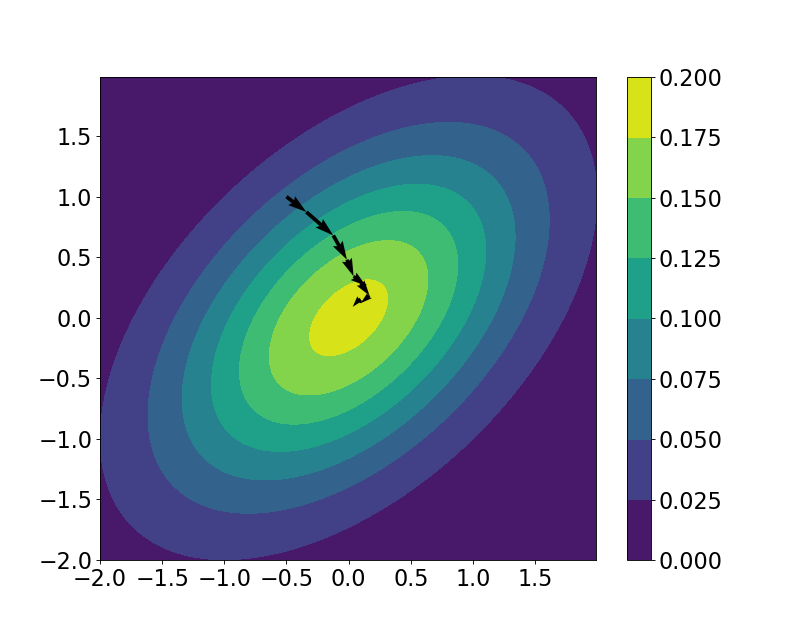
We can then view the trajectory that our “particle” took across the landscape. Plotted below is the true contour of the density of $\mu$, along with the samples from the HMC loop, plotted with arrows between successive points.

Recall that there are two main hyperparameters we have to choose in HMC: $L$, the number of leapfrog iterations, and $\epsilon$, the step size. Let’s play with these hyperparameters and see how the sample trajectories change depending on their settings.

Here’s the trajectories for the same model for three values of $\epsilon$: 0.01, 0.1, and 0.5:

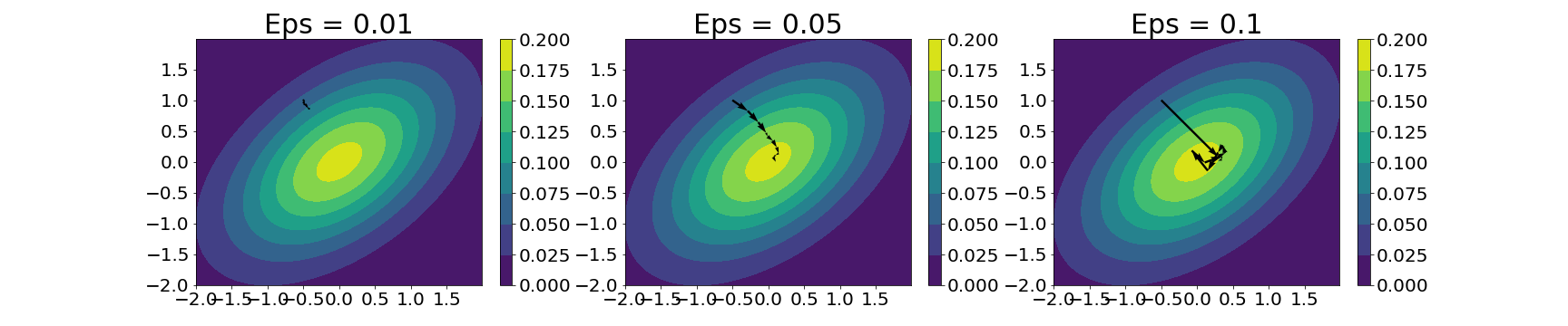
Clearly, with a lower step size, we’re allowed more precision in each of the steps, but at the cost of a slow-moving particle. With a higher step size, we can explore the landscape more, but at the cost of jumping too far in some cases.

We can do a similar experiment with the $L$ hyperparameter, here trying it with three values: $1$, $5$, and $10$:

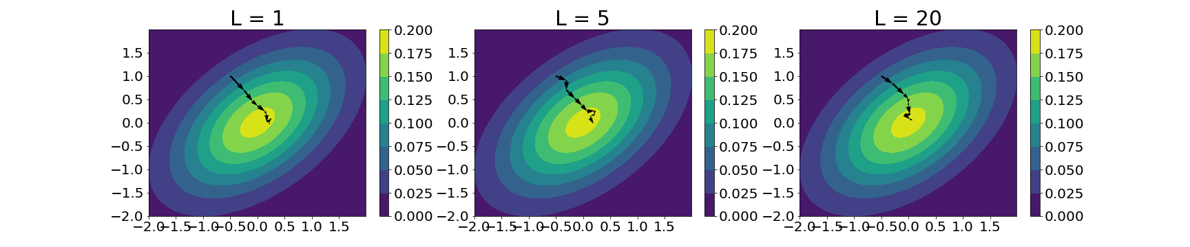
In this case, it’s less clear (at least visually) of the trade-offs implied by changing $L$. This is perhaps due to the extreme simplicity of this example. However, in general, a lower value of $L$ puts us at risk for random walk behavior, while a larger value of $L$ could result in a loop back to the starting point.

In general, setting these hyperparameters can be a tedious task. Some methods have been proposed to automatically tune them, such as the No U-Turn Sampler, which sets $L$ adaptively during the HMC sampling process.

References

• Wikipedia entry on HMC
• Betancourt, Michael. “A conceptual introduction to Hamiltonian Monte Carlo.” arXiv preprint arXiv:1701.02434 (2017).
• Hoffman, Matthew D., and Andrew Gelman. “The No-U-Turn sampler: adaptively setting path lengths in Hamiltonian Monte Carlo.” J. Mach. Learn. Res. 15.1 (2014): 1593-1623.