Andy Jones
The unintuitive nature of high-dimensional spaces
\(\DeclareMathOperator*{\argmin}{arg\,min}\) \(\DeclareMathOperator*{\argmax}{arg\,max}\)
One-, two-, and three-dimensional Euclidean spaces are easy for humans to reason about. Distances, volumes, and probability distributions are well-behaved and understandable in these low-dimensional spaces. However, this nice behavior can be deceiving. The properties of high-dimensional spaces are quite different from low-dimensional spaces, especially in the context of probability theory and statistics.
This difference primarily arises due to the unintuitive nature of high-dimensional spaces. While distances in two- and three-dimensioal spaces are easy to intuit for the human mind, imagining the distance between two points in a 10,000-dimensional Euclidean space is much less natural. To compensate, we often assume that our understanding of distances in low-dimensional space still holds for these high-dimensional spaces. Unfortunately, this is wildly wrong.
In this post, we explore some of this unintuitive behavior, with a primary focus on the implications for statistics and probability.
High-dimensional balls are mostly hollow shells
One of the most confusing things to understand about high-dimensional objects is where most of the volume of these objects lies.
To see this, let’s consider a ball in Euclidean spaces of different dimensions. Recall that a ball centered at the origin is the set of all points of distance less than a radius $r$ from the origin. We can denote this set as $\{ \mathbf{x} : ||\mathbf{x}||_2 < r\}$, where $\mathbf{x} \in \mathbb{R}^p$ is a vector. In this example, we’ll consider what happens to the volume of a thin shell at the outer part of the ball across different dimensions.
Let’s start with an extremely trivial case: the two-dimensional disk, $\{x_1, x_2 : x_1^2 + x_2^2 < r\}$. Suppose we consider the outer shell of this circle with width $\ell$, as shown in the diagram below.
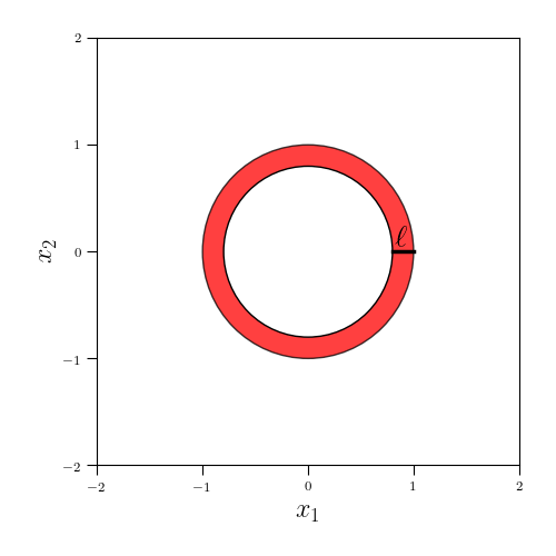
We can compute the area of this shell as the difference between the area of the outer circle and the innter circle:
\[\pi r^2 - \pi (r - \ell)^2 = 2\pi r \ell - \pi \ell^2.\]Now, moving to three dimensions, we can do the analogous calculation:
\[\frac43 \pi r^3 - \frac43 \pi (r - \ell)^3.\]And finally, let’s generalize this to a $p$-dimensional space. In this general case, the volume of a shell of width $\ell$ is
\[\frac{\pi^{p/2} r^p}{\Gamma(p / 2 + 1)} - \frac{\pi^{p/2} (r - \ell)^p}{\Gamma(p / 2 + 1)} = \frac{\pi^{p/2} (r^p - (r - \ell)^p)}{\Gamma(p / 2 + 1)}.\]For context, let’s do some simple calculations. Suppose $r = 1$ and $\ell = 0.1$. For the three-dimensional case, the volume of the shell is
\[\frac43 \pi 1^3 - \frac43 \pi (1 - 0.1)^3 = 0.419.\]As a fraction of the overall volume, this shell makes up $0.419 / 4.19$ of the ball, or approximately $10\%$.
For the 100-dimensional case, the fraction of the ball’s volume occupied the shell is given by
\[\frac{\pi^{100/2} (1^{100} - (1 - 0.1)^{100})}{\pi^{100/2} 1^{100}} = 1 - 0.9^{100} \approx 0.999.\]Thus, while our shell only makes up about $10\%$ of the ball in the three-dimensional case, it occupies nearly all of the volume in the 100-dimensional case.
In general, the fraction occupied by the shell when $r=1$ will be given by
\[1 - (1 - \ell)^p.\]As $p \to \infty$ grows, this fraction approaches $1$, meaning that, asymptotically, all of the volume lies on a thin outer shell.
If we look at the rate at which this fraction approaches $1$ with respect to $\ell$ instead, we can see that balls in higher dimesions need thinner shells to make up nearly all of their volume. The plot below shows the fraction of a $p$-dimensinoal ball’s volume occupied by a shell with width $\ell$. We keep $r=1$ here.
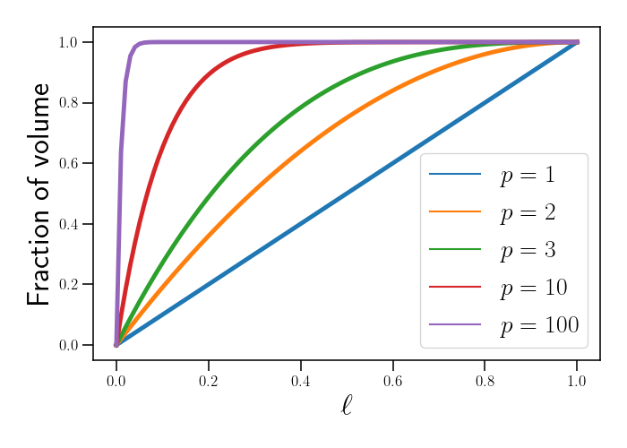
We can see that for higher values of $p$, the shell which occupies $99.99\%$ of the volume gets thinner and thinner.
This phenomenon is perhaps the most confusing part of high-dimensional spaces. Simply because of the sheer number of dimensions in a Euclidean space, the outer ring of a ball becomes massive and thereby occupies most of the volume.
High-dimensional Gaussians
In statistics, the features of high-dimensional spaces have practical consequences for modeling high-dimensional data. A common modeling assumption is that a set of data or parameters are distributed according to a multivariate Gaussian distribution.
Gaussians have tons of nice mathematical properties that make them easy to work with and that make inference and estimation straightforward. But it’s worth considering what this assumption really means in high-dimensional spaces. For example, below is a plot of the $L_2$ norm of vector drawn from a $p$-dimensional spherical Gaussian. We average over $1000$ samples here.
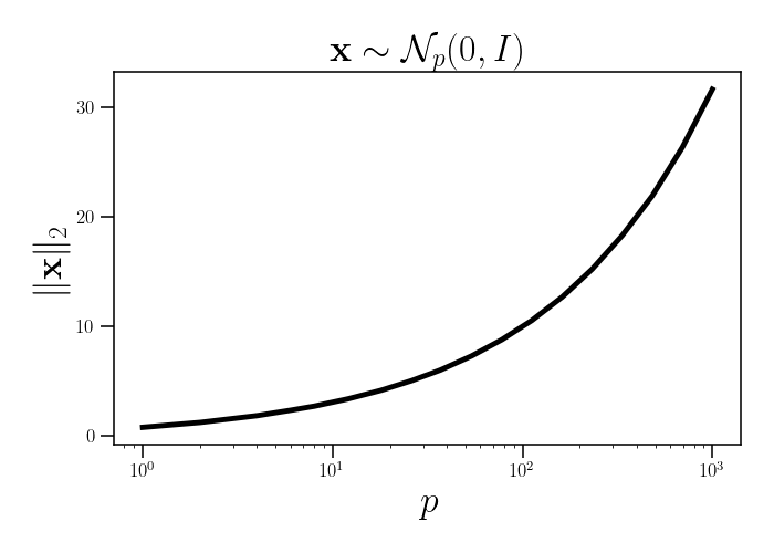
As the dimension of the Gaussian increases, the average length of a vector drawn from this distribution also increases. Although the mode of a Gaussian is always around its mean (zero in this case), the typical vector drawn from a high-dimensional Gaussian may not be close to the mean. In fact, as we saw above, the sample will most likely reside on a thin shell.
\begin{align} \mathbb{E}_{\mathbf{x} \sim \mathcal{N}_p(0, I)}[||\mathbf{x}||_2^2] &= \sum\limits_{j=1}^p \mathbb{E}_{x_j \sim \mathcal{N}(0, 1)}[x_j^2] \\ &= \mathbb{E}_{x_j \sim \mathcal{N}(0, 1)} \left[\sum\limits_{j=1}^p x_j^2 \right] \\ &= p, \end{align}
where we have used the fact that the sum of $p$ squared standard Gaussians is distributed as a $\chi^2$ random variable with $p$ degrees of freedom. In words, this means that the squared norm of a Gaussian random vector will be proportional to the dimension of the Gaussian.
This is one instance of a diffuse phenomenon that’s widely known as the “curse of dimensionality”. While there doesn’t seem to be a single agreed-upon definition for it, the term generally refers to the unintuitive behavior of high-dimensional spaces and the difficulty of accurately and efficiently modeling data in these spaces.
To consider how far astray our low-dimensional intuition can lead us in high-dimensional contexts, consider again sampling from a set of high-dimensional Gaussians (suppose $p=1,000$, for example). Here, we’ll show plots in two dimensions for clarity, although clearly this phenomenon doesn’t hold in two dimensions. This example is adapted from that of Ferenc Huszár.
What we might imagining is happening is plotted in the left panel below: three nice clouds of points, with most of the mass near the center of each cluster.
In reality, however, the right panel is closer to reality. When we sample from the Gaussians, most of the points lie on a thin ring around the mean. Again, this isn’t true in two dimensions, but we’re imagining these points are in a high-dimensional space in this exercise.
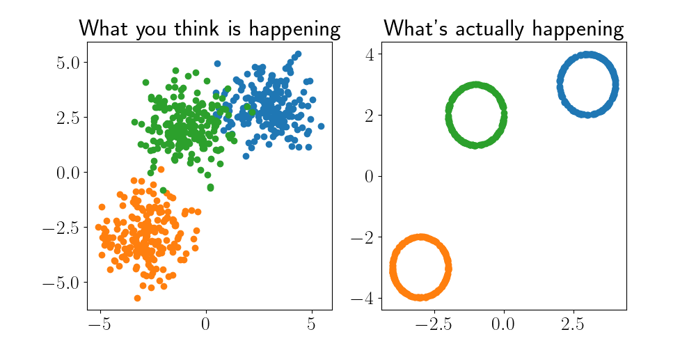
Ferenc Huszár writes that we should think of high-dimensional Gaussians as “soap bubbles”, where most of the mass is on the outer shell of the bubble.
Conclusion
While it may seem innocuous (or maybe even conservative) to make a Gaussian assumption in high-dimensional Euclidean spaces, there can be unexpected practical consequences.
References
- This StackOverflow post.
- Ferenc Huszár’s blog post