Andy Jones
Learning from Expert Advice and Hedge
Online learning algorithms make decisions in uncertain, constantly-changing environments. This post will review a couple basic forms of online learning algorithms, as well as some motivating examples.
Introduction
Imagine there are 10 stocks you’d like to invest in, and you’re seeking to maximize your profit over the next few years. Each morning before the market opens, you can choose how to allocate your money over the 10 stocks. Algorithmic results in online learning have shown that (and as we’ll see in this post), somewhat amazingly, you can devise a strategy that will perform almost as well as the best stock in the long run.
Learning from expert advice
In learning theory and algorithms classes, this type of setup falls under the umbrella of what is often called “learning from expert advice.” The generic setting is an iterative game for $T$ iterations, and in each iteration the player must make a decision (assume a binary decision for simplicity for now). The game also includes a set of $N$ experts, who give advice to the player on each iteration in the form of a suggested decision (each expert outputs $0$ or $1$ in our binary case). The player can use this advice however she likes.
To use the stock market as a motivating example, imagine predicting whether a single stock will go up or down each day. Suppose the player watches $N$ financial analysts on TV, who give their opinions on the stock’s future performance. Then, the player can decide to invest or withhold her money.
Importantly, the player’s goal in this setting is to make as few mistakes as possible, relative to the best expert. In other words, we can’t hope to get $0$ error in most settings, so we aim to perform as well as the best expert. This metric is called “regret”, and it’s calculated as the difference between the player’s error and the best expert’s.
At time $t$, let $x_t$ is the player’s decision and $y_t$ be the true label. Let $\ell_t(i)$ be the loss of expert $i$ at time $t$, where $\ell_t(i) = 1$ if the expert errs, and $\ell_t(i) = 0$ otherwise. Then the regret is
\[\text{Regret} = \sum\limits_{t = 1}^T 1[x_t \neq y_t] - \min_{i \in [N]} \sum\limits_{t = 1}^T \ell_t(i)\]where $1$ is the indicator function here.
This setting can be extended to continuous decision sets as well. Consider the example in the introduction in which there are $N$ stocks, and the player must decide how to allocate her money across the stocks. More precisely, she must choose a point on the $N$-dimensional simplex (i.e., the fraction invested in each stock must sum to $1$). In this case, we can calculate the player’s instantaneous loss as the dot product between her action $x_t$ and the experts’ losses: $x_t^\top \ell_t$. Then regret can be computed as:
\[\text{Regret} = \sum\limits_{t = 1}^T x_t^\top \ell_t - \min_{i \in [N]} \sum\limits_{t = 1}^T \ell_t(i)\]Hedge algorithm
The Hedge algorithm attempts to minimize this regret. It maintains a set of weights over experts $W_t \in \mathbb{R}^N$, where $W_t(i)$ is the weight of the $i$’th expert. Initially, all weights are set to be equal at an arbitrary value (say $1$). Then, on each iteration, the algorithm updates the weights as follows.
- Form distribution $x_t$ over experts. For each expert $i$, set $\frac{x_t(i)}{\sum_{i = 1}^N x_t(i)}$.
- Incur loss (or gain) over experts $\ell_t$.
- Update weights for all $i$: $W_{t+1}(i) = W_t(i) e^{-\epsilon \ell_t(i)}$.
This is sometimes known as the “exponential weights” algorithm because of the form of the weight update.
Intuitively, Hedge is simply downweighting the influence of the experts who tend to be wrong more often. Over time, assuming some experts are better than others, the distribution of weights will reflect the quality of the experts.
Regret of Hedge
By playing Hedge as a strategy, the player can achieve the same error as the best expert in the long run. In other words, Hedge is able to “track” the best expert.
More specifically, the expected regret is bounded as
\[\text{Regret} \leq \epsilon \sum_{t = 1}^T x_t^\top \ell_t^2 + \frac{\log N}{\epsilon}.\]To prove this, we can use a fairly straightforward series of inequalities. See Chapter 1 in Prof. Elad Hazan’s book in the references for more details.
Playing Hedge with stocks
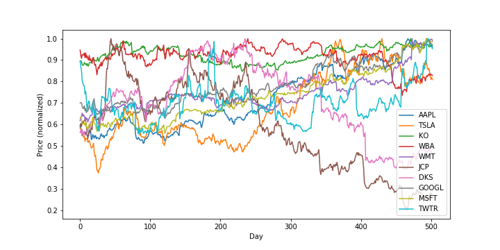
To illustrate Hedge’s strategy, let’s look at some real-world data. Here, I pulled ticker prices for 10 stocks in the years 2016-2017, which turns out to be about 500 trading days. Here are the prices over time, normalized to be in $[0, 1]$:
Now, let’s play Hedge over these $500$ days and try to track the best expert. Note that in this case, we’ll be using an (especially) unrealistic model of the stock market. Specifically, we assume that for a given day’s ticker price, the player gains that amount of money, proportional to the weight placed on that stock (i.e., there are no losses here). In reality, gain should be computed as proportional to the daily price change, not the absolute daily price, but we stick to this unrealistic model for simplicity. Additionally, note that in contrast to the algorithm statement above, we’re maximizing gain, rather than minimizing loss, but this is a trivial change.
Okay, now let’s run Hedge. Remember, the “experts” here are the stocks, and on each iteration, we’re choosing a distribution over stocks to allocate our money.
Here’s the trace of the stock weights over time:
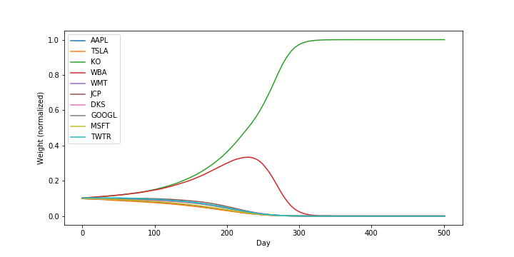
Notice that Hedge clearly picks out one stock (Coca-Cola) to allocate all of its weight after about day 250.
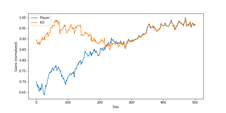
Looking at the player’s gains over time, we can see that they eventually track Coca-Cola exactly, as all weight is allocated to this stock:
Conclusion
Here, we reviewed a simple online learning algorithm called Hedge, which fits into the broader umbrella of learning with expert advice. This type of algorithm historically paved the way for more sophisticated online optimization algorithms, and many of these can be unified under a common framework called Mirror Descent. A future post will cover this framework.
References
- Hazan, Elad. “Introduction to online convex optimization.” Foundations and Trends® in Optimization 2.3-4 (2016): 157-325.
- Arora, Sanjeev, Elad Hazan, and Satyen Kale. “The multiplicative weights update method: a meta-algorithm and applications.” Theory of Computing 8.1 (2012): 121-164.
- My lecture notes from Prof. Hazan’s Theoretical Machine Learning course.
- Freund, Yoav, and Robert E. Schapire. “A decision-theoretic generalization of on-line learning and an application to boosting.” Journal of computer and system sciences 55.1 (1997): 119-139.