Gaussian process latent variable models

\(\DeclareMathOperator*{\argmin}{arg\,min}\) \(\DeclareMathOperator*{\argmax}{arg\,max}\)

Dimensionality reduction is useful for understanding the broad patterns in a high-dimensional dataset. Many of the most common techniques – such as PCA and factor analysis – assume that the true data manifold is a linear subspace. However, this assumption of linearity can be overly strong in most cases.

A swarm of nonlinear dimensionality reduction methods have been developed in the past couple decades. Here, we review an important method that has its origins in the probabilistic modeling community: the Gaussian process latent variable model (GPLVM). Below, we first show how the GPLVM is related to probabilistic PCA, and then we review the details of the model and associated inference.

Probabilistic PCA

Recall the generative model for probabilistic PCA (PPCA) for zero-mean data $x \in \mathbb{R}^D$:

\begin{align} x &= Wz + \epsilon \\ z &\sim \mathcal{N}(0, I_d) \\ \epsilon &\sim \mathcal{N}(0, \sigma^2 I_D) \end{align}

where $z \in \mathbb{R}^{d}$ is a latent variable. We assume $d < D$.

Inference typically proceeds by marginalizing out $z$ and maximizing the resulting likelihood with respect to $W$ and $\sigma^2$. The marginal distribution of $x$ is

Given an $D \times N$ data matrix $X$, the MLE for $W$ can be found by maximizing this likelihood:

where $A = WW^\top + \sigma^2 I$. This can be solved analytically. Denote the eigendecomposition of the sample covariance as $X^\top X = U\Lambda U^\top$. Then, the MLE solution is

\begin{align} \widehat{W}_{MLE} &= U_d \left( \Lambda_d - \sigma^2 I \right)^{1/2} R \\ \widehat{\sigma^2}_{MLE} &= \frac{1}{D - d} \sum\limits_{j = d + 1}^D \lambda_j \end{align}

where the columns of $U_d$ contain the leading $d$ eigenvectors of $X^\top X$, $\Lambda_d$ is a diagonal matrix containing the leading $d$ eigenvalues, and $R$ is any $d \times d$ orthogonal rotation matrix. Intuitively, we can think of the MLE solution for $W$ as very similar to the solution of non-probabilistic PCA, but adjusted for the noise $\sigma^2$.

PPCA provides a nice, simple latent variable model interpretation for PCA. It also provides much of the groundwork and intuition for GPLVMs, which we explore next.

GPLVM

The GPLVM has a similar motivation to PPCA: to find a low-dimensional representation of the data that retains the important characteristics. However, while PPCA assumed a linear mapping between the latent space and the data space, the GPLVM allows nonlinear mappings. By placing a (nonparametric) GP prior over this function $f : \mathbb{R}^d \rightarrow \mathbb{R}^D$, the GPLVM allows for more flexible representations.

Mathematically, we can start by viewing the GPLVM as a “dual” version of PPCA. Instead of marginalizing out $z,$ (as above) we can marginalize out $W$. In this model, we place a conjugate Gaussian prior on $W$ and treat $z$ as a parameter to be estimated. The corresponding generative model is as follows:

\begin{align} x &= Wz + \epsilon \\ p(W) &= \prod_{j=1}^D \mathcal{N}(w_j | 0, I) \\ \epsilon &\sim \mathcal{N}(0, \sigma^2 I_D). \end{align}

Note that we still have the assumption of linearity, but we’ll relax this in a moment. The resulting marginal likelihood is also Gaussian:

As above, suppose we have $N$ samples arranged in the rows of a matrix $X \in \mathbb{R}^{N \times D}$ with corresponding latent variables $Z \in \mathbb{R}^{N \times d}$. (Note that we transposed the data matrix here for convenience.) Let the eigendecomposition of the Gram matrix be $X X^\top = U\Lambda U^\top.$ Then, we can solve for the MLE of the latent variables $Z$. The log likelihood of the data is given by

The solution is given by

where the columns of $U_d \in \mathbb{R}^{n \times d}$ contain the leading $d$ eigenvectors of $X X^\top$, and $\Lambda_d$ is a diagonal matrix containing the leading $d$ eigenvalues of $X X^\top$.

Notice that the above solution required us to compute a measure of (dis)similarity between all pairs of latent variables. In this case, the covariance was defined by the linear covariance, $ZZ^\top + \sigma^{-2} I,$ which, in vector form, corresponds to the kernel function $k(z, z^\prime) = zz^\prime.$ However, this is just one specific choice for $k$, but we can choose many others, as we’ll see next.

Generalizing the kernel $K$

We sometimes call the covariance matrix the “kernel” matrix, denoted by $K$. In the linear formulation above, we had $K = ZZ^\top + \sigma^{-2} I$. However, as hinted above, we can generalize this using any valid PSD kernel function. In this case, we define the matrix as $[K]_{ij} = k(z_i, z_j).$ For instance, a common choice is the RBF kernel:

Notice that this kernel function resembles the Gaussian PDF, and indeed corresponds to the assumption that the similarity between random variables falls off exponentially fast as the distance between them increases.

Maximum likelihood estimation

Under the GPLVM, the likelihood of the data is

where $\theta$ represents the kernel hyperparameters and $K_{ZZ}$ is the kernel evaluated at all pairs of latent variables,

Our goal is then to maximize this likelihood with respect to $Z$ and $\theta$,

\begin{align} (Z_{MLE}, \theta_{MLE}) &= \argmax_{Z, \theta} \left\{ p(X | Z, \theta) \right\} \\ &= \argmax_{Z, \theta} \left\{ \log p(X | Z, \theta) \right\} \\ &= \argmax_{Z, \theta} \left\{ \log \prod\limits_{j=1}^D (2\pi)^{-N/2} |K_{ZZ}|^{-1/2} \exp\left\{ -\frac12 x_j^\top K_{zz}^{-1} x_j \right\} \right\} \\ &= \argmax_{Z, \theta} \left\{ -\frac{DN}{2} \log 2\pi - \frac{D}{2} \log |K_{ZZ}| - \frac12 X^\top K_{ZZ}^{-1} X \right\}. \end{align}

There isn’t a closed-form solution to this problem, but we can use gradient-based methods to estimate $Z$ and $\theta$. Instead, we can take the derivative of the above likelihood $L$ with respect to the kernel matrix, $\frac{\partial L}{\partial K}$, and combine that with the deriviative of $K$ with respect to the latent variables $Z$, $\frac{\partial K}{\partial Z}$. First, we have

This comes from the derivative of each term in the log likelihood above:

\begin{align} \frac{\partial}{\partial K} \left( -\frac{DN}{2} \log 2\pi \right) &= 0 \\ \frac{\partial}{\partial K} \left( - \frac{D}{2} \log |K| \right) &= - DK^{-1} \\ \frac{\partial}{\partial K} \left(- \frac12 X^\top K^{-1} X \right) &= K^{-1} XX^\top K^{-1}. \\ \end{align}

The derivative $\frac{\partial K}{\partial Z}$ will depend on the specific choice of the kernel function. If we choose a linear kernel function, we recover the PPCA model and solution, which has a closed form. While it’s possible to derive other kernel-specific derivatives by hand, it’s much more common in practice to rely on automatic differentiation tools. These tools also allow for easily trying different kernel functions without having to re-derive the gradient updates. Below, we show a simple example of doing this.

Example

To show the GPLVM in action, let’s consider a simple two-dimensional example. Suppose the relationship between the columns of our data is a quadratic function,

Here’s a plot of our data, with additive Gaussian noise:

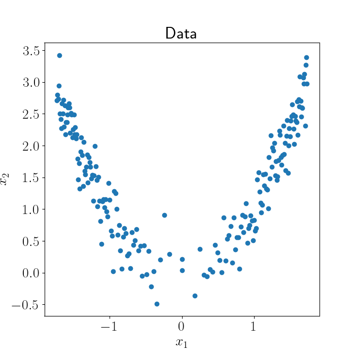
Here, it’s clear that our data isn’t actually “two-dimensional” in some sense. Rather, we can describe our data fairly well with just a one-dimensional curve, although this curve won’t be a straight line. A GPLVM can help us find this curve.

Let’s show this by fitting a GPLVM in Python. Here, we’ll use autograd to optimize the log marginal likelihood with respect to the latent variables. We’ll use an RBF kernel, but we won’t optimize the kernel parameters just for simplicity. All of the code is available in the Code section, but I’ll provide a short walk-through of the code here.

First, we can write down our objective function. In this case, it corresponds to the negative log marginal likelihood (negative because we’ll seek to minimize our objective). We can use some built-in Python functions to compute this, placing an isotropic Gaussian prior on the latent variables:

def gaussian_log_likelihood(X, mean, covariance, sigma2=1):
	ll = np.sum([mvn.logpdf(X[:, ii], mean, covariance) for ii in range(D)])
	return ll

def gaussian_prior(Z):
	covariance = np.eye(n)
	mean = np.zeros(n)
	ll = np.sum([mvn.logpdf(Z[:, ii], mean, covariance) for ii in range(d)])
	return ll

def objective(Z):
	# The objective is the negative log likelihood of the data.
	Z = np.reshape(Z, (n, d))
	cov_mat = kernel(Z, Z) + np.eye(n)
	ll = gaussian_log_likelihood(X, zero_mean, cov_mat)
	lprior = gaussian_prior(Z)
	return -(ll + lprior)

Furthermore, we can define the RBF kernel:

def rbf_kernel(x1, x2, sigma2=1, lengthscale=1):
	output_scale = 1
	lengthscales = 1
	diffs = np.expand_dims(x1 / lengthscale, 1)\
		  - np.expand_dims(x2 / lengthscale, 0)
	return np.exp(-0.5 / sigma2 * np.sum(diffs**2, axis=2))

Finally, we can initialize our latent variables randomly and minimize the objective using scipy’s minimize function:

init_params = np.random.normal(size=(n * d))
res = minimize(value_and_grad(objective), init_params, jac=True, method='CG')
fitted_Z = np.reshape(res.x, (n, d))

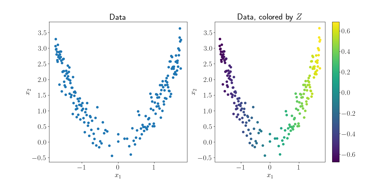
Now, we can examine the MLE for the latent variables. First, let’s plot the final fitted values. Below, the left plot shows the original data. The right plot is the same data, where we’ve colored each point by the value of its associated latent variable. As expected, we find that the GPLVM can recover the underlying parabolic curve of the data, as indicated by the continuous gradient of color across the curve

We can also observe the iterative process of fitting the GPLVM. The animation below shows each step of the minimization of the objective. The left plot is again the data colored by the associated latent variable value. On the right, we plot $x_1$ (the first data dimension) against the value of the latent variables.

We can see that the GPLVM quickly identifies the curve underlying our data.

References

• Lawrence, Neil, and Aapo Hyvärinen. “Probabilistic non-linear principal component analysis with Gaussian process latent variable models.” Journal of machine learning research 6.11 (2005).
• Lawrence, Neil D. “Gaussian process latent variable models for visualisation of high dimensional data.” Nips. Vol. 2. 2003.
• Some of my code is based off of the autograd GPLVM implementation.

Code

import numpy as onp
import matplotlib.pyplot as plt
import seaborn as sns
from autograd import grad, value_and_grad
import autograd.numpy as np
from autograd.misc.optimizers import adam
import autograd.scipy.stats.multivariate_normal as mvn
from scipy.optimize import minimize

inv = np.linalg.inv
import matplotlib
font = {"size": 20}
matplotlib.rc("font", **font)
matplotlib.rcParams["text.usetex"] = True

def make_parabola_data(n=100, sigma2=1):
	x1 = np.sqrt(np.linspace(0, 3, n//2))
	x1 = np.concatenate([-x1, x1])
	x1 = np.sort(x1)
	x2 = x1**2 + np.random.normal(scale=np.sqrt(sigma2), size=n)
	return np.vstack([x1, x2]).T

def rbf_kernel(x1, x2):
	output_scale = 1
	lengthscales = 1
	diffs = np.expand_dims(x1 / lengthscales, 1)\
		  - np.expand_dims(x2 / lengthscales, 0)
	return output_scale * np.exp(-0.5 / 10 * np.sum(diffs**2, axis=2))

def linear_kernel(x1, x2):
	return x1 @ x2.T

def gaussian_log_likelihood(X, mean, covariance, sigma2=1):
	ll = np.sum([mvn.logpdf(X[:, ii], mean, covariance) for ii in range(D)])
	return ll

def gaussian_prior(Z):
	covariance = np.eye(n)
	mean = np.zeros(n)
	ll = np.sum([mvn.logpdf(Z[:, ii], mean, covariance) for ii in range(d)])
	return ll

def objective(Z):
	# The objective is the negative log likelihood of the data.
	Z = np.reshape(Z, (n, d))
	cov_mat = kernel(Z, Z) + np.eye(n)
	ll = gaussian_log_likelihood(X, zero_mean, cov_mat)
	lprior = gaussian_prior(Z)
	return -(ll + lprior)


fig = plt.figure(figsize=(12,8), facecolor='white')
data_ax = fig.add_subplot(121, frameon=False)
latent_ax = fig.add_subplot(122, frameon=False)
plt.show(block=False)

def callback(params):
	print('Log likelihood: {0:1.3e}'.format(-objective(params)))

	Z = np.reshape(params, (n, d))

	data_ax.cla()
	data_ax.scatter(X[:, 0], X[:, 1], c=Z[:, 0])
	data_ax.set_title('Observed Data')
	data_ax.set_xlabel(r"$x1$")
	data_ax.set_ylabel(r"$x2$")

	latent_ax.cla()
	latent_ax.plot(X[:, 0], Z[:, 0], 'kx')
	latent_ax.set_xlim([-2, 2])
	latent_ax.set_ylim([-2, 2])
	latent_ax.set_xlabel(r"$x1$")
	latent_ax.set_ylabel(r"$z$")
	latent_ax.set_title('Latent coordinates')

	plt.draw()
	plt.pause(1.0/60.0)

n = 200
D = 2
d = 1
zero_mean = np.zeros(n)
X = make_parabola_data(n=n, sigma2=0.1)

kernel = rbf_kernel
init_params = np.random.normal(size=(n * d))

res = minimize(value_and_grad(objective), init_params, jac=True, method='CG', callback=callback)
fitted_Z = np.reshape(res.x, (n, d))