Andy Jones
Generating random samples from probability distributions
I take for granted that I can easily generate random samples from a variety of probability distributions in NumPy, R, and other statistical software. However, the process for generating these quantities is somewhat nontrivial, and we’ll look under the hood at one example in this post.
Where does the randomness come from?
To be able to draw a random sample from a distribution, we first need some source of randomness. This typically comes from a pseudorandom number generator. However, these generators can only sample from one probability distribution: the uniform distribution. Although the uniform is directly useful for lots of purposes, we often need to sample from more interesting distributions, like the Gaussian. Unfortunately, there’s no pseudorandom number generator to directly sample Gaussian-distributed numbers.
One solution to this problem is to use the randomness inherent in the uniform numbers to generate arbitrary distributions. In particular, once we have uniform random samples, we could somehow transform these samples to reflect the desired distribution. So a generic recipe for generating samples from a distribution $\mathcal{D}$ is:
- Generate $X \sim \text{Unif}(0, 1)$ using a pseudorandom number generator.
- Transform $X$ to have distribution $\mathcal{D}$.
A general rule: the probability integral transform
A general method for transforming uniform random variables to another arbitrary distribution is the probability integral transform. This transform uses the basic property of cumulative distribution functions that their percentiles are uniformly distributed. In particular, consider any random variable $X$ with a valid CDF $F_X(x)$. Then $Y = F_X(x)$ has a uniform distribution (recall that $F_X(x) = \mathbb{P}[X \leq x]$, and probabilities are always in the interval $[0, 1]$). So if $Y$ is uniformly distributed, and then we can just take the inverse to conclude that $F_X^{-1}$ has distribution $F_X$. Said another way, if $U \sim \text{Unif}(0, 1)$, and you’d like to transform $U$ to a distribution with CDF $F_X$, then the random variable $F_X^{-1}(U)$ will have distribution $F_X$. This already gives us a way to leverage the pseudorandom number generator to sample from more interesting distributions.
For example, consider an exponentially-distributed random variable $X \sim \text{Exp}(\lambda)$. The CDF of $X$ is $F_X(x) = 1 - e^{-\lambda x}$, and its inverse is $F_X^{-1}(y) = -\lambda \log(1 - y)$. If we plug in our uniform random variable $U \sim \text{Unif}(0, 1)$ as $y$, we would receive an exponentially-distributed random variable.
However, the probability integral transform doesn’t always work because $F_X^{-1}$ may have a nasty form for many distributions, or it may not have a closed form at all.
Generating Gaussian RVs: the Box-Muller algorithm
One example where applying the probability integral transform coule be tricky is transforming a uniform to a Gaussian. The following Gaussian integral doesn’t have a nice closed form:
\[\int_{-\infty}^\infty e^{\frac{-x^2}{2}} dx.\]However, clearly, it’s very important to have easy (and quick) ways to generate samples from the Gaussian. One clever solution for doing this is the Box-Muller algorithm. The key idea here is that although sampling one Gaussian random variable is difficult, sampling two is actually easier. Consider two independent standard normals:
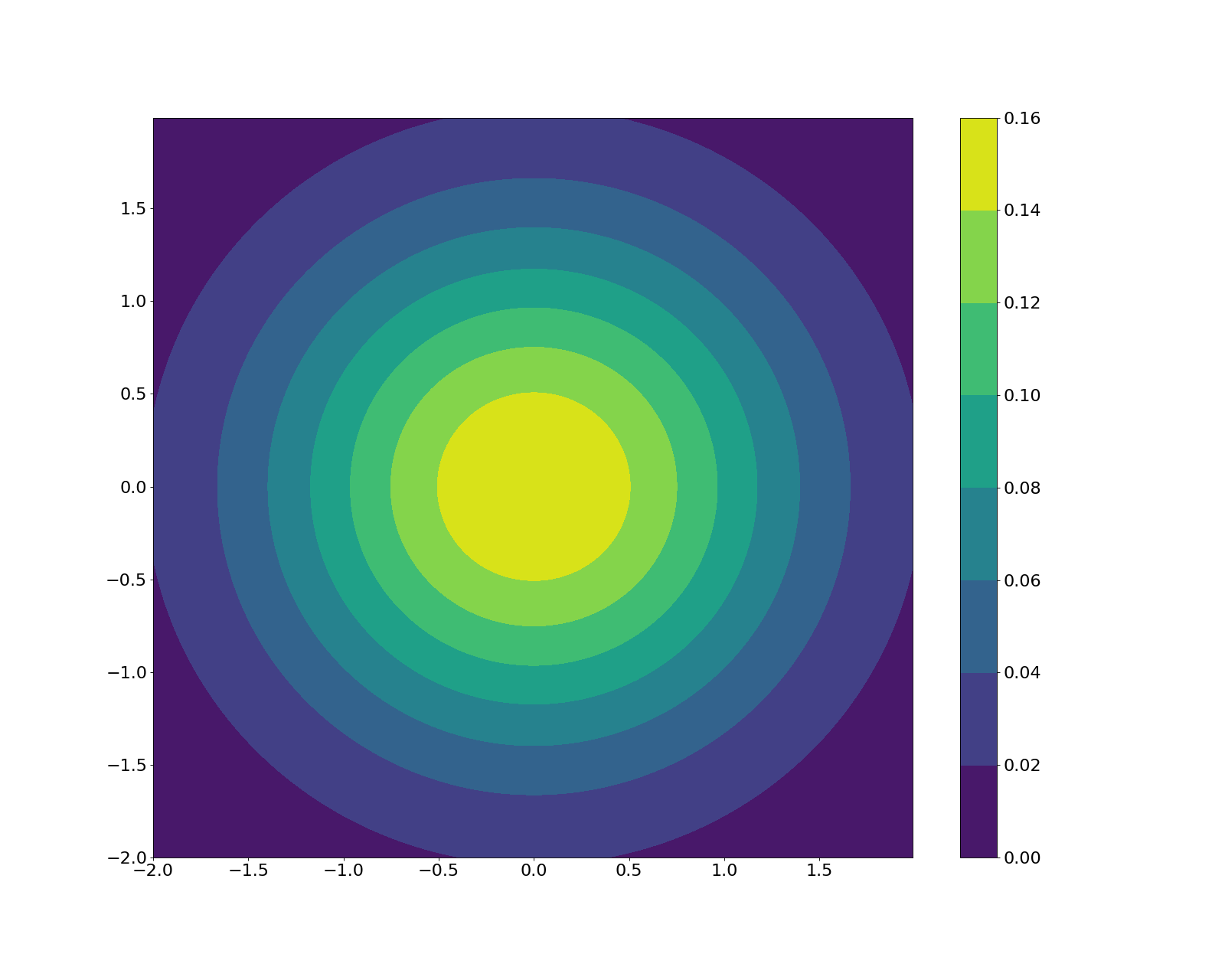
They’re clearly radially symmetric. Again, it’s difficult to directly sample from this distribution, but there is another way we could sample a point around this circle according to the Gaussian density – using polar coordinates!
In order to sample a polar coordinate, we need an angle $\theta$ around the origin, and a number $R$ representing the point’s distance from the origin. Once we have these, we can transform back to cartesian with the familiar form: $X = R\cos \theta$ and $Y = R\sin \theta$. But first, we have to find a way to sample $\theta$ and $R$ appropriately.
Since the 2D Gaussian is radially symmetric, we can sample $\theta$ uniformly from $[0, 2\pi]$. That is, if $U_1$ is a uniform random number in $[0, 1]$, then $\theta = 2\pi U_1$ is a uniform random number in $[0, 2\pi]$.
To sample $R$, we can use the probability integral transform (full circle!). Recall that in order to do this, we need to find its CDF and then its inverse. Luckily, unlike the Gaussian integral above, we can solve this one! The CDF for $R$ is
\[\mathbb{P}[R \leq r] = \int_{r' = 0}^r \int_{\theta = 0}^{2\pi} e^{-r'^2/2} rdrd\theta = 1 - e^{-r^2 / 2}.\]See Prof. Noah Goodman’s lecture notes for a simple way to compute this with change of variables.
Now, by the probability integral transform, $1 - e^{-r^2 / 2}$ must have a uniform distribution, so we can solve for a transformation from a uniform random variable $U_2$ to $R$. Note that $1 - U_2$ is also uniform, so we can plug that in instead in order to get rid of the $1$ floating around. Solving, we now have a way to compute $R$:
\[R = \sqrt{-2 \log U_2}.\]Putting it all together, here’s the recipe for generating two independent Gaussian random variables $X$ and $Y$:
- Generate two uniform random numbers $U_1, U_2$ from $[0, 1]$ using a pseudorandom number generator.
- Set $\theta = 2 \pi U_1$.
- Set $R = \sqrt{-2 \log U_2}$.
- Generate $X = R \cos \theta$, $Y = R \sin \theta$.
This is called the Box-Muller transform, and it’s widely used, including in NumPy’s sampler.
Just to prove to ourselves that it works, let’s run a simulation. If we run the recipe above 1000 times, here’s the distribution we get for the resulting 2000 samples:
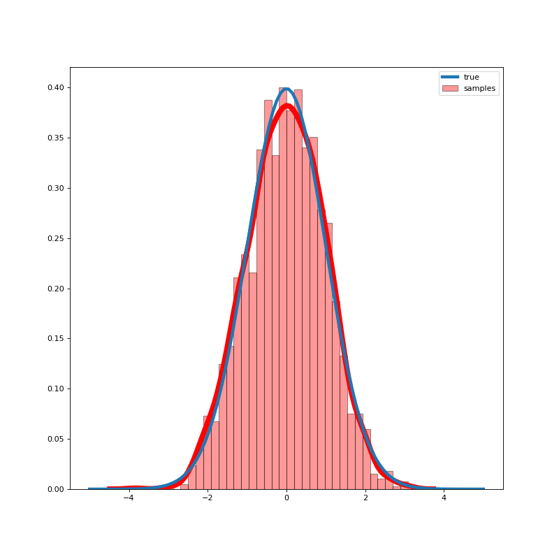
The theoretical standard normal distribution is in blue, and our estimate is in red. Pretty good!
Of course, this is just for sampling from the standard normal $\mathcal{N}(0, 1)$. If we want to sample more generally from $\mathcal{N}(\mu, \sigma^2)$, we can scale and shift appropriately. Specifically, if $Z \sim \mathcal{N}(0, 1)$, then $X = \sigma Z + \mu$ has distribution $\mathcal{N}(\mu, \sigma^2)$.
Conclusion
Here, we partially demystified how software packages sample from non-uniform distributions of random variables and studied the special case of the Gaussian.
References
- Casella, G. and R. L. Berger (2002): Statistical Inference, Duxbury.
- Prof. Noah Goodman’s lecture notes on Monte Carlo methods
- Wikipedia entries for probability integral transform and Box-Muller transform