Gaussian process regression

A brief review of Gaussian processes with simple visualizations.

Introduction

A Gaussian process is a stochastic process $\mathcal{X} = \{x_i\}$ such that any finite set of variables $\{x_{i_k}\}_{k=1}^n \subset \mathcal{X}$ jointly follows a multivariate Gaussian distribution:

According to Rasmussen and Williams, there are two main ways to view Gaussian process regression: the weight-space view and the function-space view. Here, we consider the function-space view.

In the function-space view of Gaussian process regression, we can think of a Gaussian process as a prior distribution over continuous functions. Specifically, consider a regression setting in which we’re trying to find a function $f$ such that given some input $x$, we have $f(x) \approx y$.

In a parametric regression model, we would specify the functional form of $f$ and find the best member of that family of functions according to some loss function. For example, we might assume that $f$ is linear ($y = x \beta$ where $\beta \in \mathbb{R}$), and find the value of $\beta$ that minimizes the squared error loss using the training data ${(x_i, y_i)}_{i=1}^n$:

Gaussian process regression offers a more flexible alternative, which doesn’t restrict us to a specific functional family. Instead, we specify relationships between points in the input space, and use these relationships to make predictions about new points.

In particular, consider the multivariate regression setting in which the data consists of some input-output pairs ${(\mathbf{x}_i, y_i)}_{i=1}^n$ where $\mathbf{x}_i \in \mathbb{R}^p$ and $y_i \in \mathbb{R}$. Generally, our goal is to find a function $f : \mathbb{R}^p \mapsto \mathbb{R}$ such that $f(\mathbf{x}_i) \approx y_i \;\; \forall i$.

In Gaussian process regress, we place a Gaussian process prior on $f$,

where $\mu(\mathbf{x})$ is the mean function, and $k(\mathbf{x}, \mathbf{x}^\prime)$ is the kernel function.

By placing the GP-prior on $f$, we are assuming that when we observe some data, any finite subset of the the function outputs $f(\mathbf{x}_1), \dots, f(\mathbf{x}_n)$ will jointly follow a multivariate normal distribution:

where we use Rasmussen’s notation where

and $K(\mathbf{X}, \mathbf{X})$ is a matrix of all pairwise evaluations of the kernel matrix:

Note that WLOG we assume that the mean is zero (this can always be achieved by simply mean-subtracting).

Drawing from the GP prior

We can sample from the prior by choosing some values of $\mathbf{x}$, forming the kernel matrix $K(\mathbf{X}, \mathbf{X})$, and sampling from the multivariate normal.

We can show a simple example where $p=1$ and using the squared exponential kernel in python with the following code.

# Draw x samples
n = 100

for _ in range(10):
    X = np.linspace(-5, 5, n)

    # Form covariance matrix between samples
    K = np.zeros((n, n))

    for ii in range(n):
        for jj in range(n):
            curr_k = kernel(X[ii], X[jj])
            K[ii, jj] = curr_k
            K[jj, ii] = curr_k


    # Draw Y from MVN
    Y = mvn(mean=np.zeros(n), cov=K, allow_singular=True).rvs()

The resulting draws look like this:

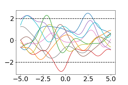
The two dotted horizontal lines show the $2 \sigma$ bounds.

Predictions in GP regression

Given some training data, we often want to be able to make predictions about the values of $f$ for a set of unseen input points $\mathbf{x}^\star_1, \dots, \mathbf{x}^\star_m$. GPs make this easy by taking advantage of the convenient computational properties of the multivariate Gaussian distribution.

Given the training data $\mathbf{X} \in \mathbb{R}^{n \times p}$ and the test data $\mathbf{X^\star} \in \mathbb{R}^{m \times p}$, we know that they are jointly Guassian:

We can visualize this relationship between the training and test data using a simple example with the squared exponential kernel. Consider the case when $p=1$ and we have just one training pair $(x, y)$. Suppose $x=2.3$. Without considering $y$ yet, we can visualize the joint distribution of $f(x)$ and $f(x^\star)$ for any value of $x^\star$.

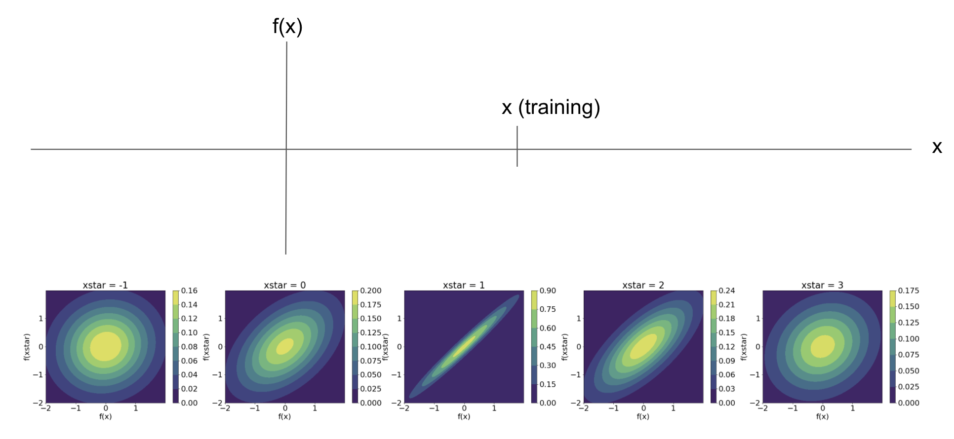
As we can see, the joint distribution becomes much more “informative” around the training point $x=1.2$. In other word, as we move away from the training point, we have less information about what the function value will be.

Now, suppose we observe the corresponding $y$ value at our training point, so our training pair is $(x, y) = (1.2, 0.9)$, or $f(1.2) = 0.9$ (note that we assume noiseless observations for now). For any test point $x^\star$, we are interested in the distribution of the corresponding function value $f(x^\star)$. Thus, we are interested in the conditional distribution of $f(x^\star)$ given $f(x)$.

Recall that if two random vectors $\mathbf{z}_1$ and $\mathbf{z}_2$ are jointly Gaussian with

then the conditional distribution $p(\mathbf{z}_1 | \mathbf{z}_2)$ is also Gaussian with

Applying this to the Gaussian process regression setting, we can find the conditional distribution $f(\mathbf{x}^\star) | f(\mathbf{x})$ for any $\mathbf{x}^\star$ since we know that their joint distribution is Gaussian. In particular, if we denote $K(\mathbf{x}, \mathbf{x})$ as $K_{\mathbf{x} \mathbf{x}}$, $K(\mathbf{x}, \mathbf{x}^\star)$ as $K_{\mathbf{x} \mathbf{x}^\star}$, etc., it will be

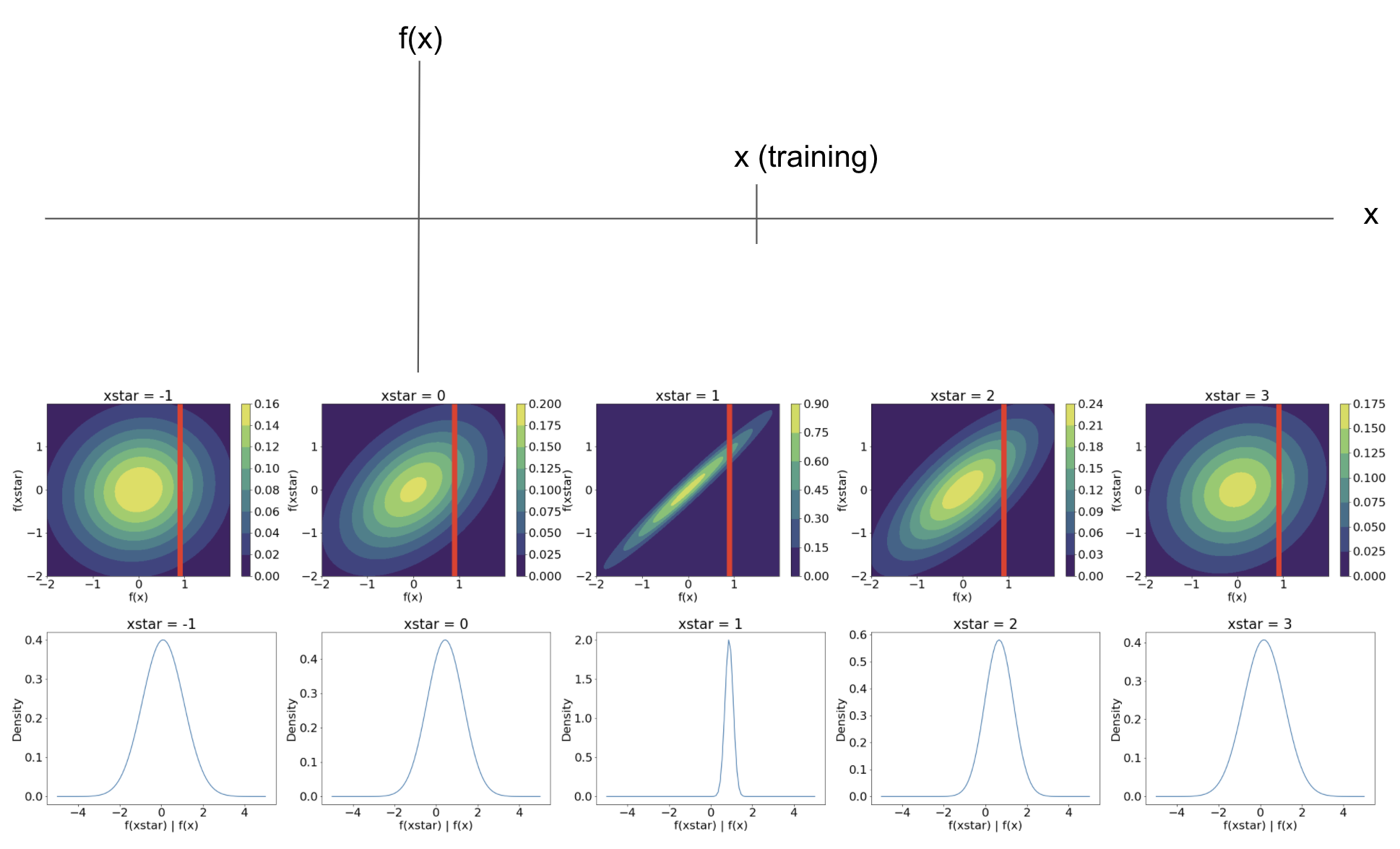
Using our simple visual example from above, this conditioning corresponds to “slicing” the joint distribution of $f(\mathbf{x})$ and $f(\mathbf{x}^\star)$ at the observed value of $f(\mathbf{x})$. Below is a visualization of this when $p=1$. The vertical red line corresponds to conditioning on our knowledge that $f(1.2) = 0.9$. In the bottom row, we show the distribution of $f^\star | f$. Notice that it becomes much more peaked closer to the training point, and shrinks back to being centered around $0$ as we move away from the training point.

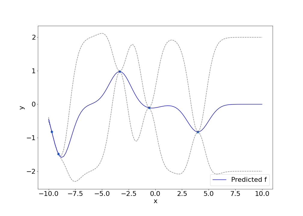
Now, consider an example with even more data points. Suppose we observe the data below.

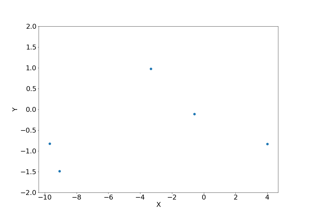
We can predict densely along different values of $x^\star$ to get a series of predictions that look like the following. The blue dots are the observed data points, the blue line is the predicted mean, and the dashed lines are the $2\sigma$ error bounds.

Conclusion

Gaussian process regression offers a more flexible alternative to typical parametric regression approaches. Its computational feasibility effectively relies the nice properties of the multivariate Gaussian distribution, which allows for easy prediction and estimation.

References

• Rasmussen, Carl Edward. “Gaussian processes in machine learning.” Summer School on Machine Learning. Springer, Berlin, Heidelberg, 2003.
• Prof William Welch’s notes on the multivariate Gaussian

Code

Kernels:

### Kernels

def gaussian_kernel(x1, x2):
    return np.exp(-0.5 * (x1 - x2)**2)


def linear_kernel(x1, x2):
    return x1 * x2

kernel = gaussian_kernel

Drawing from GP prior:

# Draw x samples
n = 100

for _ in range(10):
    X = np.linspace(-5, 5, n)

    # Form covariance matrix between samples
    K = np.zeros((n, n))

    for ii in range(n):
        for jj in range(n):
            curr_k = kernel(X[ii], X[jj])
            K[ii, jj] = curr_k
            K[jj, ii] = curr_k


    # Draw Y from MVN
    Y = mvn(mean=np.zeros(n), cov=K, allow_singular=True).rvs()
    
    plt.plot(X, Y)

plt.axhline(-2, linestyle='--', c='black')
plt.axhline(2, linestyle='--', c='black')
plt.savefig("./out/gp_prior_draws.png")
plt.show()

Visualizing joint distributions:

# Example with one observed point and varying test point

import matplotlib
font = {'size'   : 22}

matplotlib.rc('font', **font)

xtrain, ytrain = 1.2, 0.9

plt.figure(figsize=(45, 6))
xstar_list = [-1, 0, 1, 2, 3]
for iter_num, xstar in enumerate(xstar_list):
    
    # Get kernel matrix
    K = np.array([
        [kernel(xtrain, xtrain), kernel(xtrain, xstar)],
        [kernel(xstar, xtrain), kernel(xstar, xstar)]
    ])
    
    x, y = np.mgrid[-2:2:.01, -2:2:.01]
    pos = np.empty(x.shape + (2,))
    pos[:, :, 0] = x; pos[:, :, 1] = y
    rv = mvn(np.zeros(2), cov=K)
    
    
    plt.subplot(1, len(xstar_list), iter_num + 1)
    plt.contourf(x, y, rv.pdf(pos))
    cbar = plt.colorbar()
    plt.title("xstar = {}".format(xstar))
    plt.xlabel("f(x)")
    plt.ylabel("f(xstar)")
    plt.axvline(ytrain, c='red', linewidth=10)
            

plt.savefig("./out/joint_prior_dist.png")
plt.show()

Predictions in GP regression:

# Gaussian process regression

plt.figure(figsize=(14, 10))
# Draw function from the prior and take a subset of its points

left_endpoint, right_endpoint = -10, 10

# Draw x samples
n = 5
X = np.random.uniform(low=left_endpoint, high=right_endpoint, size=n)

# Form covariance matrix between samples
K11 = np.zeros((n, n))
for ii in range(n):
    for jj in range(n):
        curr_k = kernel(X[ii], X[jj])
        K11[ii, jj] = curr_k

# Draw Y from MVN
Y = mvn(mean=np.zeros(n), cov=K11, allow_singular=True).rvs()

plt.scatter(X, Y, s=50)


# Get predictions at a dense sampling of points
nstar = 100
Xstar = np.linspace(left_endpoint, right_endpoint, nstar)


# Form covariance matrix between test samples
K22 = np.zeros((nstar, nstar))
for ii in range(nstar):
    for jj in range(nstar):
        curr_k = kernel(Xstar[ii], Xstar[jj])
        K22[ii, jj] = curr_k
        
# Form covariance matrix between train and test samples
K12 = np.zeros((n, nstar))
for ii in range(K12.shape[0]):
    for jj in range(K12.shape[1]):
        curr_k = gaussian_kernel(X[ii], Xstar[jj])
        K12[ii, jj] = curr_k
        
K21 = K12.T


# Get predictive distribution mean and covariance

def matrix_inverse(A):
    c = np.linalg.inv(np.linalg.cholesky(A))
    inverse = np.dot(c.T,c)
    return inverse

Ystar_mean = K21 @ matrix_inverse(K11) @ Y
Ystar_cov = K22 - K21 @ matrix_inverse(K11) @ K12

# Sample
Ystar = mvn(mean=Ystar_mean, cov=Ystar_cov, allow_singular=True).rvs()

# plt.plot(Xstar, Ystar, c='r', label="True f")

plt.plot(Xstar, Ystar_mean + 2 * np.diagonal(Ystar_cov), linestyle='--', color='gray')
plt.plot(Xstar, Ystar_mean - 2 * np.diagonal(Ystar_cov), linestyle='--', color='gray')

plt.plot(Xstar, Ystar_mean, c="blue", label="Predicted f")

plt.xlabel("x")
plt.ylabel("y")
plt.legend()

plt.savefig("./out/gp_predictions.png")
plt.show()