The forward-backward algorithm

\(\DeclareMathOperator*{\argmin}{arg\,min}\) \(\DeclareMathOperator*{\argmax}{arg\,max}\)

Problem setup

Consider a hidden Markov model (HMM) for a sequence of length $n.$ Denote the data (emission) and latent variable on step $i$ as $x_i$ and $z_i,$ respectively. We denote the entire set of data and latent variables as $X = (x_1, \dots, x_n)$ and $Z = (z_1, \dots, z_n).$

Suppose there are $K$ possible latent states, and a latent variable can transition between these states on each step. Let $A$ be the matrix of transition probabilities where $A_{ij}$ represents the probability of transitioning from state $i$ to state $j,$ and let $\phi$ be the parameters for the emission model. The likelihood of the data and latent variables is given by

Computing the posterior

Suppose we would like to compute the marginal posterior distribution for one latent variable, $p(z_i | X).$ The forward-backward algorithm is one approach for doing this.

Using Bayes rule, we can write the marginal posterior for $z_i$ as

We can rewrite the numerator of this posterior as a product of two terms: one that depends only on time steps on or before $i$ and another that depends only on time steps on or after $i.$ We do this as follows:

\begin{align} p(X | z_i) p(z_i) &= p(x_1, \dots, x_n | z_i) p(z_i) & \text{(Write out $x$’s)} \\ &= p(x_1, \dots, x_i | z_i) p(x_{i+1}, \dots, x_n | z_n) p(z_i) & \text{($d$-separation)} \\ &= \color{blue}{p(x_1, \dots, x_i, z_i)} \color{orange}{p(x_{i+1}, \dots, x_n | z_i)}, \end{align}

where on the last step we have simply collapsed the conditional probability. We now assign names to these two expressions:

\begin{align} \color{blue}{\alpha(z_i)} &\color{blue}{= p(x_1, \dots, x_i, z_i)} \
\color{orange}{\beta(z_i)} &\color{orange}{= p(x_{i+1}, \dots, x_n | z_i)}. \end{align}

Computing $\alpha(z_i)$ and $\beta(z_i)$ correspond to the forward and backward steps of the forward-backward algorithm, respectively. As we’ll see next, this is because computing $\alpha(z_i)$ requires recursively stepping through the sequence forward, and computing $\beta(z_i)$ requires recursively stepping backward.

Forward pass

To begin to compute $\alpha(z_i),$ let’s first show how we can write $\alpha(z_i)$ recursively in terms of $\alpha(z_{i-1}).$ The following sequence of identities uses the principle of $d$ separation as well as the basic laws of probability:

\begin{align} \color{blue}{\alpha(z_i)} &= p(x_1, \dots, x_i, z_i) \\ &= p(x_1, \dots, x_i | z_i) p(z_i) \\ &= p(x_i | z_i) p(x_1, \dots, x_{i-1} | z_i) p(z_i) \\ &= p(x_i | z_i) p(x_1, \dots, x_{i-1}, z_i) \\ &= p(x_i | z_i) \sum_{z_{i-1}} p(x_1, \dots, x_{i-1}, z_{i-1}, z_i) \\ &= p(x_i | z_i) \sum_{z_{i-1}} p(x_1, \dots, x_{i-1}, z_i | z_{i-1}) p(z_{i-1}) \\ &= p(x_i | z_i) \sum_{z_{i-1}} p(x_1, \dots, x_{i-1} | z_{i-1}) p(z_i | z_{i-1}) p(z_{i-1}) \\ &= p(x_i | z_i) \sum_{z_{i-1}} p(x_1, \dots, x_{i-1}, z_{i-1}) p(z_i | z_{i-1}) \\ &= \color{blue}{p(x_i | z_i) \sum_{z_{i-1}} \alpha(z_{i-1}) p(z_i | z_{i-1})}. \end{align}

We now have a recursive expression for the $\alpha$ (forward) terms. To complete the computation for $i > 1,$ we need to define a base case for $\alpha(z_1).$ This is given by

Backward pass

We now compute the $\beta$ terms for the backward pass.

\begin{align} \color{orange}{\beta(z_i)} &= p(x_{i+1}, \dots, x_n | z_i) \\ &= \sum_{z_{i+1}} p(x_{i+1}, \dots, x_n, z_{i+1} | z_i) \\ &= \sum_{z_{i+1}} p(x_{i+1}, \dots, x_n | z_i, z_{i+1}) p(z_{i+1} | z_i) \\ &= \sum_{z_{i+1}} p(x_{i+2}, \dots, x_n | z_{i+1}) p(x_{i+1} | z_{i+1}) p(z_{i+1} | z_i) \\ &= \color{orange}{\sum_{z_{i+1}} \beta(z_{i+1}) p(x_{i+1} | z_{i+1}) p(z_{i+1} | z_i)}. \end{align}

This gives us a recursive expression for the $\beta$ (backward) terms. To get a base case for $\beta(z_n)$, we have

\begin{align} p(z_n | X) &= \frac{\alpha(z_n) \beta(z_n)}{p(X)} \\ &= \frac{p(x_1, \dots, x_n, z_n) \beta(z_n)}{p(X)} \\ &= \frac{p(X, z_n) \beta(z_n)}{p(X)}, \end{align}

which implies that $\beta(z_n) = 1.$

Completing the posterior

Recall from above that the posterior for the $i$th latent variable is given by

At this point we’re able to compute $\alpha(z_i)$ and $\beta(z_i),$ but we still have to compute $p(X).$ Since the posterior is discrete, we can easily solve for it by simply computing the normalizing constant, which is given by

Avoiding numerical underflow

Each step of computing $\alpha$ and $\beta$ requires multiplying numbers that are less than one. Thus, for long sequences, these numbers will become very small and could cause problems for machine precision. To alleviate this, $\alpha(z_i)$ and $\beta(z_i)$ are commonly normalized on each step so that $\sum_{z_i} \alpha(z_i) = \sum_{z_i} \beta(z_i) = 1.$

Demonstration

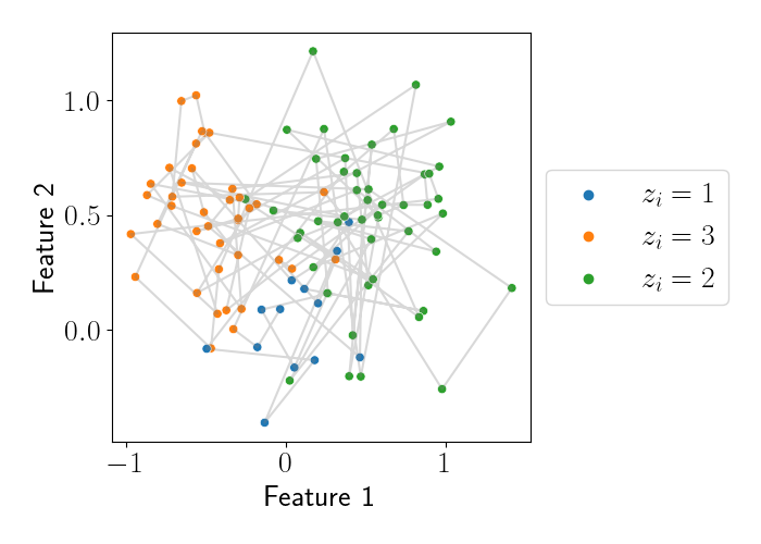
Let’s now show a simple demonstration with simulated data. Consider a sequence of length $n=100$ where there are assumed to be $K=3$ latent states. We will assume that each data point (emission) is a bivariate Gaussian random variable with isotropic covariance, so the emission model is given by

where $\mu_k \in \mathbb{R}^2$ is a latent-state-specific mean parameter, and $\sigma^2_k$ is a latent-state-specific covariance parameter. For the purposes of this demonstration, we assume that these parameters are known with $\mu_1 = (0, 0)^\top,$ $\mu_2 = (0.5, 0.5)^\top,$ $\mu_3 = (-0.5, 0.5)^\top,$ and $\sigma^2_1 = \sigma^2_2 = \sigma^2_3 = 0.1.$ We set the (known) transition matrix to be

In other words, for each state there is an $80\%$ probability of staying in that state and a $10\%$ chance of moving to either of the other two states.

We set $z_1 = 1$ and simulate data for this model. The Python code below performs this simulation.

import numpy as np
import matplotlib.pyplot as plt
import seaborn as sns
from os.path import join as pjoin
from scipy.stats import multivariate_normal as mvn

# Sequence length
n = 100

# Number of latent states
K = 3

# Emission parameters
emission_means = np.array(
    [
        [0, 0],
        [0.5, 0.5],
        [-0.5, 0.5]
    ]
)
emission_vars = np.array([0.1, 0.1, 0.1])

# Transition probabilities
tprob_self = 0.8
A = np.array(
    [
        [tprob_self, (1 - tprob_self) / 2, (1 - tprob_self) / 2],
        [(1 - tprob_self) / 2, tprob_self, (1 - tprob_self) / 2],
        [(1 - tprob_self) / 2, (1 - tprob_self) / 2, tprob_self],
    ]
)

# Priors
pi = np.ones(K) / K

# Simulate data from model
np.random.seed(1)
zs = np.zeros(n).astype(int)
xs = np.zeros((n, 2))
zs[0] = 0
xs[0] = mvn.rvs(mean=emission_means[zs[0]], cov=emission_vars[zs[0]] * np.eye(2))

for ii in range(1, n):
    zs[ii] = np.random.choice(np.arange(K), p=A[zs[ii - 1]])
    xs[ii] = mvn.rvs(mean=emission_means[zs[ii]], cov=emission_vars[zs[ii]] * np.eye(2))

The data is plotted below, where each point is colored by its latent variable assignment, and the gray lines connect successive points in the sequence.

Using these data, let’s try to estimate the posterior for the latent variables $Z = (z_1, \dots, z_{100}).$ To start, let’s compute the $\alpha$ values. The code below does this.

# Initialize
alphas = np.zeros((n, K))

# Base case
alphas[0] = pi * [mvn.pdf(xs[0], mean=emission_means[zz], cov=emission_vars[zz] * np.eye(2)) for zz in range(K)]
alphas[0] /= alphas[0].sum()

# Start recursion
for ii in range(1, n):
    likelihoods = np.array([mvn.pdf(xs[ii], mean=emission_means[zz], cov=emission_vars[zz] * np.eye(2)) for zz in range(K)])
    transition_probs = A @ alphas[ii - 1]
    alphas[ii] = likelihoods * transition_probs
    alphas[ii] /= alphas[ii].sum()

We can then compute the $\beta$ terms with the code below.

# Initialize
betas = np.zeros((n, K))

# Base case
betas[-1] = np.ones(K)
betas[-1] /= betas[-1].sum()

# Start recursion
for ii in np.arange(len(betas) - 2, -1, -1):
    
    likelihoods = np.array([mvn.pdf(xs[ii + 1], mean=emission_means[zz], cov=emission_vars[zz] * np.eye(2)) for zz in range(K)])
    transition_probs = A @ betas[ii + 1]
    betas[ii] = likelihoods * transition_probs
    betas[ii] /= betas[ii].sum()

We then compute the posterior probabilities by taking the product of the $\alpha$ and $\beta$ terms for each step and then normalizing them.

posterior_probs_unnormalized = alphas * betas
posterior_probs = posterior_probs_unnormalized / posterior_probs_unnormalized.sum(axis=1)[:,None]

We can then plot the posterior at each sequence index for each possible latent state. The plot below shows this, where each line tracks the posterior distribution for one latent state, and the dots at the top show the true latent state.

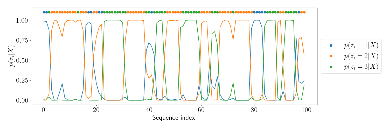
We can see that the posterior closely aligns with the true latent variable value, especially for parts of the sequence with longer repeats. For indices in which there is a repeat of just one latent variable value, the posterior places less weight on the true value.

References

• Bishop, Christopher M., and Nasser M. Nasrabadi. Pattern recognition and machine learning. Vol. 4. No. 4. New York: springer, 2006.