Andy Jones
Epistemic and aleotoric uncertainty in statistical models
\(\DeclareMathOperator*{\argmin}{arg\,min}\) \(\DeclareMathOperator*{\argmax}{arg\,max}\)
When we make a prediction about the world, there is always going to be some amount of uncertainty in that prediction. This uncertainty can be roughly broken down into two types: epistemic uncertainty and aleotoric uncertainty.
These two types are roughly defined as follows.
- Epistemic uncertainty refers to incomplete knowledge about the true state of the world.
- Aleotoric uncertainty, on the other hand, refers to the inherent noise or randomness in a phenomenon.
In this post, we’ll try to break down these dense definitions into understandable explanations and visualizations.
Visualizing epistemic and aleotoric uncertainty
Consider the following dataset consisting of $30$ observations of two variables, $x$ and $y$:
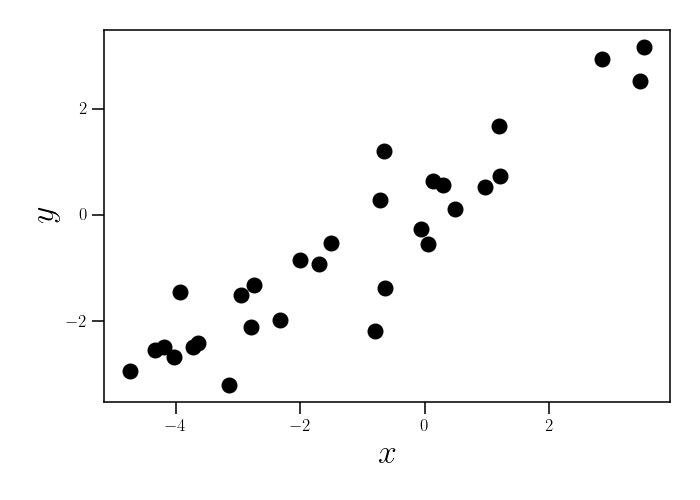
After a simple glance at the data, it seems reasonable to model the relationship between $x$ and $y$ with a linear function. In particular, suppose we posit the following model for the data:
\begin{equation} y = x \beta + \epsilon,~~~\epsilon \sim \mathcal{N}(0, \sigma^2). \label{eq:linear_model} \tag{1} \end{equation}
In this setting, our epistemic uncertainty is embedded in the linear model itself. For this reason, epistemic uncertainty is also sometimes called model uncertainty. By positing a linear model for these data, we’re making a fairly strong assumption about the relationship between $x$ and $y$. But how do we know that the data don’t actually arise from a different type of model. We don’t (at least with finite data), and this is the source of epistemic uncertainty.
To visualize this, what if, instead of a linear model, the data actually arose from a periodic function? Or a cubic function? Or some other crazy function? Furthermore, even within the linear model class, we may not be entirely sure which value of $\beta$ best fits the data.
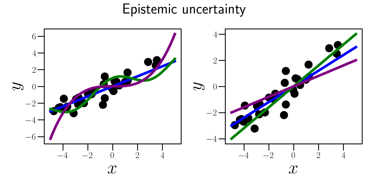
Although some of these functions might seem implausible upon initial inspection, we can’t be 100% certain in our choice of model with a finite dataset. However, as we’ll see below, the epistemic uncertainty disappears as we go to the limit of infinite data.
Now, let’s visualize the source of aleotoric uncertainty. Suppose we fit our linear model, finding the value of $\beta$ that best describes our data. Even with the best model parameter $\beta$, our linear model doesn’t capture the full variation in the data. Specifically, there is still noise around the regression line. This is the source of aleotoric uncertainty, as shown below.
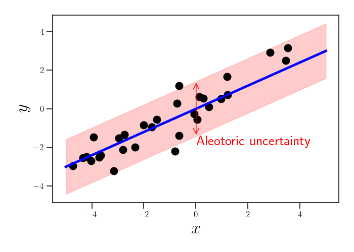
Notice that, even if we collected infinite data, our aleotoric uncertainty would never disappear. Said another way, if we want to predict $y$ given a new value of $x$, our prediction accuracy will be limited by our amount of aleotoric uncertainty. This source of uncertainty is captured by $\sigma^2$ in our linear model (Equation \ref{eq:linear_model}).
Bayesian vs. Frequentist uncertainty
The way we think about epistemic and aleotoric uncertainty is slightly different between frequentist and Bayesian realms. Above, we took a frequentist approach, modeling the data as random samples from a linear model. Our epistemic uncertainty was hard-coded into the model in that case.
In a Bayesian approach, our epistemic uncertainty is also partially encoded in the prior distribution. To see this, let’s put a Bayesian spin on our previous linear model. Let’s now consider the following model:
\begin{align} y &= x \beta + \epsilon \\ \beta &\sim \mathcal{N}(0, 1) \\ \epsilon &\sim \mathcal{N}(0, \sigma^2). \end{align}
The only difference between this model and the previous one is that now we have a distribution over our regression coefficient $\beta$. A Bayesian would then perform inference by computing the posterior of $\beta$ given the data. In this simple model, the posterior has a closed form. Let $\mathbf{x} = (x_1, \cdots, x_n)^\top$ and $\mathbf{y} = (y_1, \cdots, y_n)^\top$ be vectors containing the data. Then the posterior is given by:
\[\beta | \mathbf{x}, \mathbf{y} \sim \mathcal{N}\left(\frac{\mathbf{x}^\top \mathbf{y}}{\sigma^2 + \mathbf{x}^\top \mathbf{x}}, \frac{1}{1 + \frac{1}{\sigma^2} \mathbf{x}^\top \mathbf{x}}\right).\]Let’s visualize the posterior for $\beta$ as the dataset size increases. Below, in the left panel we plot a streaming dataset, where the dataset size increases from $1$ to $100$. In blue, we plot the line given by the posterior mean for $\beta$. In the right panel, we show the posterior $p(\beta | \mathbf{x}, \mathbf{y})$ for each dataset. The true value of $\beta^\star=0.6$ is shown by a green dashed line.
We can see that the posterior contracts around $\beta^\star$ as the dataset size increases. We can roughly think of the width of this posterior as an estimate of the magnitude of our epistemic uncertainty. As we observe more data, we become more and more certain about the true model, meaning that our epistemic uncertainty declines (and eventually vanishes).
Debate over usefulness of distinction
There is some debate over the usefulness and aptness of the distinction between epistemic and aleotoric uncertainty. Some people argue that all uncertainty is simply a product of having incomplete information about some phenomenon, and that any distinction between two types of missing information is a false dichotomy. It is relatively uncontroversial that epistemic uncertainty arises from incomplete information. After all, we saw that as we get more data (information), this type of uncertainty disappears.
However, aleotoric uncertainty can be much more elusive context-dependent. In our linear regression example, where did the aleotoric uncertainty actually arise from. If $y$ is a noisy measurement from a physical sensor, then our aleotoric uncertainty arises because of this noise. But, assuming there is enough information in the world to eventually characterize this noise process, isn’t this just another case of incomplete information?
As we can see, the distinction between these two types of uncertainty isn’t rigid and often depends on the context of the model and the phenomenon that’s being studied. What we choose to treat as epistemic vs. aleotoric uncertainty will often depend on our goals. We may choose to model one specific relationship between a set of variables, and try to soak up any remaining variation with a “noise” model.
References
- David Aldous’s notes on the topic.
- Kendall, Alex, and Yarin Gal. “What uncertainties do we need in bayesian deep learning for computer vision?.” Advances in neural information processing systems 30 (2017).