Andy Jones
Gibbs posteriors and energy-based models
\(\DeclareMathOperator*{\argmin}{arg\,min}\) \(\DeclareMathOperator*{\argmax}{arg\,max}\)
A common critique of the Bayesian approach to statistical inference is its dogmatic reliance on specific probability models for data. If all models are incorrect in some way or another, the critique goes, why should we trust inferences made from these models?
In response to this, there have been several attempts in recent years to make probabilistic modeling more flexible and to leverage some of the advances in machine learning to allow for more data-driven learning, as opposed to requiring full model specification from the start.
In this post, we give a brief overview of some of the approaches to generalize Bayesian posterior inference in order to make it more flexible for modern data types. Specifically, we focus on Gibbs posteriors and energy-based models, which rely on the same building blocks, although they arose in different schools of thought.
The statistical physics point-of-view
Approaches to flexibly modeling probability distributions first arose in the statistical physics community. In these problems, physicists were considering physical systems containing multiple objects, each of which had an energy associated with it. The scientists were then interested in characterizing the probability that the physical system would be in any given overall state (i.e., any single combination of each object’s state).
To formalize the problem a bit more, let’s consider an example. Suppose we have two particles, each of which has a one-dimensional position (state) associated with it within some spatial domain $\mathcal{X}.$ Denote the particles’ postitions as $x_1, x_2 \in \mathcal{X},$ and their vector as $\mathbf{x} = (x_1, x_2)^\top.$ Each state configuration has a different energy associated with it. Let $E : \mathcal{X}^2 \to \mathcal{E}$ be a function that maps the configuration to an energy within the domain $\mathcal{E} \subset \mathbb{R}.$ Suppose we’d like to understand the probability that the two particles will reside in a certain state.
It turns out that this probability is given by the Gibbs-Boltzmann distribution
\[p(\mathbf{x}) = \frac{\exp\left\{-\frac1T E(\mathbf{x})\right\}}{Z},\]where $T$ is the temperature of the system, and $Z = \int_{\mathcal{X}^2} \exp\left\{-\frac1T E(\mathbf{x})\right\} d\mathbf{x}$ is a normalizing constant that makes the distribution sum to one. (Technically, we should also include a term for the Boltzmann constant, but we have omitted that here, or we can imagine it being absorbed into the temperature.) In our two-particle example, the function $E$ would only take two possible values, but one can imagine the energy function being much more general.
Thus, the Gibbs-Boltzmann distribution gives us a route to convert energy function (whose range could be the whole real line) into a probability density function (which must sum to one by definition).
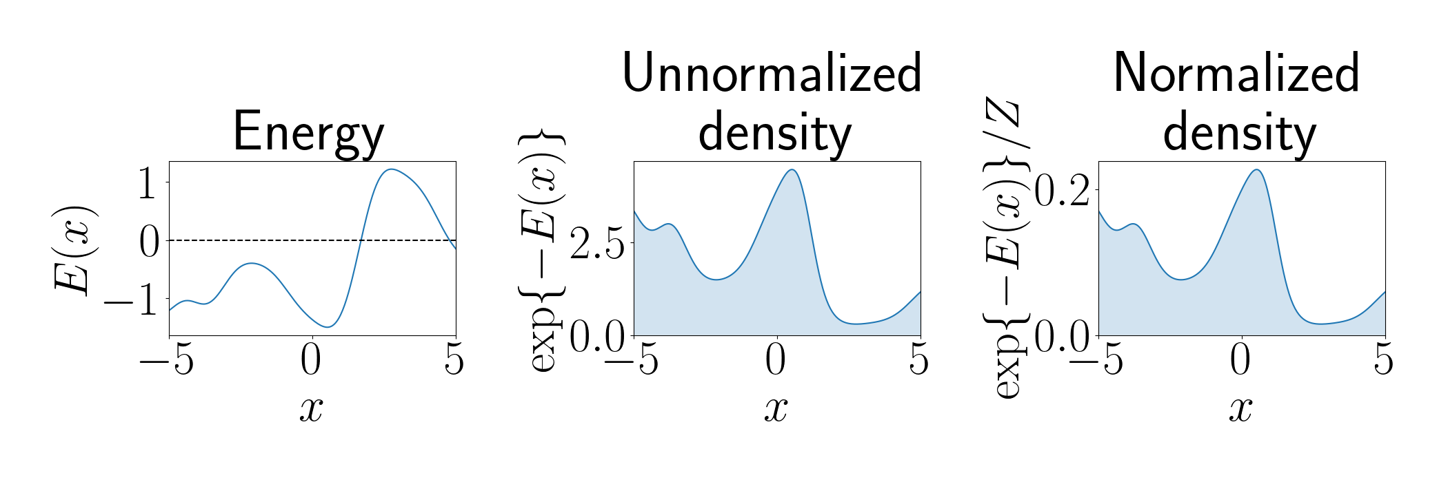
The plot below shows a demonstration of going from an energy function to a normalized density using the Gibbs-Boltzmann distribution. The left panel shows an energy function where $x$ is a one-dimensional state. The middle panel shows the unnormalized density, and the right panel shows the normalized density.
We can immediately draw two conclusions from the Gibbs-Boltzmann distribution:
- States with lower energy will have higher probabilities;
- A higher temperature will make the distribution more peaked around its modes, and a lower temperature will flatten the distribution (notice that if we let $T \to 0,$ then all states are assigned equal probability).
To demonstrate the role of the temperature parameter, the animation below shows the normalized density for a range of temperatures from $T=0$ to $T=10.$
Moving beyond the physics perspective, let’s now look at how these ideas can be useful for statistical inference.
Gibbs posteriors
Recall the form of Bayes theorem for computing the posterior of a parameter $\theta$ given data $x:$
\[p(\theta | x) = \frac{p(x | \theta) p(\theta)}{p(x)}.\]Application of Bayes theorem to statistical inference requires us to choose the likelihood function $p(x | \theta),$ which describes the likelihood of observing $x$ under parameter setting $\theta.$ In real world applications, it is essentially impossible to correctly specify this function, and often the choice is made primarily based on computational convenience.
Consider a more general way of viewing the likelihood: it’s a function that links the parameter $\theta$ to the data $x.$ Framed this way, it’s not clear why the likelihood should be restricted to be a probability density function. For complex natural phenomena, choosing a likelihood PDF may be unnecessarily restrictive.
Instead, we can consider more general ways of describing the link between the parameter and the data. Consider a general “loss function” $\ell_\theta : \mathcal{X} \to \mathbb{R},$ which is parameterized by $\theta$ and measures the compatibility between the data and parameter.
Since the loss function is no longer restricted to be a PDF, we now need a way to translate the loss function into probability terms. A natural way to do this is through the Gibbs-Boltzmann distribution. This is the central idea behind the “Gibbs posterior,” which is given by
\[p(\theta | x) = \frac{\exp\{-\omega \ell_\theta(x)\} p(\theta)}{Z},\]where $\omega$ is often called the learning rate or the inverse temperature because of its relationship to the temperature parameter from the Gibbs-Boltzmann distribution, $\omega = \frac1T.$
Note that we can recover the traditional Bayesian posterior by choosing the loss function to be the negative log likelihood: $\ell_\theta(x) = -\log p(x | \theta).$ Thus, the Gibbs posterior is strictly more general than the Bayesian posterior and is sometimes called a “generalized” posterior.
While the normalizing constant $Z$ will usually be intractable for most loss functions, we can still estimate the posterior through MCMC sampling approaches that only require a quantity that is proportional to the posterior (i.e., the numerator).
Energy-based models
In the machine learning community, similar ideas have arisen under the category of energy-based models (EBMs). As the name suggests, EBMs are inspired directly by the statistical physics energy-centric perspective on probability.
The primary hallmark of EBMs is using modern ML architectures to parameterize the energy function and modern training and optimization techniques for inference.
EBMs use the same Gibbs-Boltzmann distribution as before,
\[p(x) = \frac{\exp\{-\omega E_\theta(x)\}}{Z},\]where $E_\theta(x)$ can now be parameterized with any function approximator (denoted by $\theta$ in our example). For example, $E_\theta(x)$ could be represented by a deep neural network. The advantage is that EBMs can leverage the encoding output by modern ML architectures, but convert the outputs to probabilities.
The most straightforward way to fit an EBM is to maximize the log likelihood of the data under the EBM. Specifically, the optimization problem in this approach for data $x_1, \dots, x_n$ is
\[\max_\theta \sum\limits_{i=1}^n \log p(x_i) = \min_\theta \sum\limits_{i=1}^n \left\{\omega E_\theta(x_i) + \log Z\right\}.\]In this case, we can’t ignore the normalizing constant during optimization because it depends on $\theta.$ This is again the most difficult part of fitting EBMs. In some cases, the integral inside $Z$ can be approximated directly through sampling or other approaches. A wide range of other, non-maximum-likelihood-based training strategies have also been proposed to circumvent this problem.
Demonstration
We now provide a simple demonstration of using EBMs for density estimation in Python. We consider the setting of one-dimensional density estimation: given samples $x_1, \dots, x_n$ drawn from some true (unknown) distribution $p_{data}(x),$ we’d like to estimate the density using an EBM. In this case, we’ll consider the simple example where the true data distribution is a univariate Gaussian:
\[x_1, \dots, x_n \sim \mathcal{N}(\mu, \sigma^2).\]We’ll parameterize our energy function with a cubic polynomial:
\[E_\theta(x) = a + bx + cx^2 + dx^3,\]where our optimization goal is to estimate the parameters $\theta = (a, b, c, d).$ (Note that if we parameterized the energy function with a quadratic function, then the Gibbs-Boltzmann distribution would reduce back to a Gaussian.)
While there are many ways to fit an EBM, we’ll use the maximum likelihood objective and use an extremely simple approach to estimate the normalizing constant. Since we’re considering a one-dimensional dataset with a bounded domain in this example, we’ll simply estimate the integral with the trapezoidal rule.
The code below implements this example.
import numpy as np
from scipy.optimize import minimize

lim = 5
n = 300
true_mean = 1
true_stddev = .5
X = np.random.normal(loc=true_mean, scale=true_stddev, size=n)
X = np.sort(X).reshape(-1, 1)

learning_rate = 1

def log_energy_function(theta, x):
    design_mat = np.hstack([x ** kk for kk in range(len(theta))])
    return design_mat @ theta

def partition_function(theta):
    ps = np.exp(-learning_rate * log_energy_function(theta, X))
    Z_est = np.trapz(ps, X.squeeze())
    return Z_est

def neg_log_likelihood(theta, learning_rate=1):
    return np.sum(log_energy_function(theta, X) + np.log(partition_function(theta)))

theta0 = np.random.normal(size=4)
res = minimize(fun=neg_log_likelihood, x0=theta0)
Below is an animation that shows the learned normalized density over iterations of training in orange. The blue curve shows the true data distribution from which the data were generated.
References
- LeCun, Yann, et al. “A tutorial on energy-based learning.” Predicting structured data 1.0 (2006).
- Song, Yang, and Diederik P. Kingma. “How to train your energy-based models.” arXiv preprint arXiv:2101.03288 (2021).
- Syring, Nicholas, and Ryan Martin. “Gibbs posterior concentration rates under sub-exponential type losses.” arXiv preprint arXiv:2012.04505 (2020).