Determinental point processes

\(\DeclareMathOperator*{\argmin}{arg\,min}\) \(\DeclareMathOperator*{\argmax}{arg\,max}\)

Determinental point processes (DPPs) are a class of mathematical and statistical models that are used to model general sets based on the determinant of the correlation or covariance function between the sets’ elements. In applications, they have been used in text summarization, pose estimation, and modeling repulsion of objects.

We start with a basic primer on determinants and then describe DPPs.

Geometric intuition for determinants

Recall the geometric meaning of a matrix determinant: it represents the “size” or “volume” of the linear map described by the determinant. This is most easily demonstrated in two dimensions. Consider the $2 \times 2$ matrix $A,$

The determinant is given by $\text{det}(A) = |ad - bc|.$ Geometrically, this formula is equivalent to the area of a parallelogram whose vertices are given by $(0, 0), (a, b), (c, d),$ and $(a + c, b + d).$

In other words, we can view the determinant as the area of the parallelogram induced when the unit square is transformed by a matrix $A.$ We demonstrate this visually below.

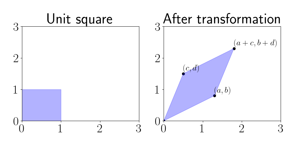
Above, we start with the unit matrix $M$ on the left. We can represent $M$ by placing the vertices’ locations as rows in a matrix:

When we transform $M$ as $MA,$ we have

The rows of this new matrix are the vertices of the parallelogram in the right panel of the plot above. The area of this parallelogram will vary depending on the elements of $A.$ Thus, one way to interpret the determinant is by how “big” the parallelogram induced by $A$’s transformation is.

Determinental point processes

We now describe determinental point processes, which use matrix determinants to quantify the probability of sets.

Consider a ground set $\Omega$ and a finite point process $\mathcal{Y},$ which is a random subset $\mathcal{Y} \subseteq \Omega.$ In this post, we’ll assume $\Omega$ is discrete and $|\Omega| = n,$ although DPPs can be applied to continuous sets as well. In the discrete case, the point process $\mathcal{Y}$ is a distribution over all subsets of $\Omega,$ denoted as $2^\Omega.$

We can form an $n \times n$ kernel matrix $\mathbf{K},$ with $\mathbf{0} \preceq \mathbf{K} \preceq \mathbf{I},$ where element $[\mathbf{K}]_{ij}$ intuitively represents the similarity between elements $i$ and $j$ of $\Omega.$ This matrix can be formed by an established correlation or covariance function, or customly constructed for a particular application.

A determinental point process arises if the probability that a subset $A \subseteq \Omega$ is in the random set $\mathcal{Y}$ is equal to the determinant of the submatrix of $\mathbf{K}$ corresponding to these elements. More concretely, let $\mathbf{K}_A$ be the submatrix of $\mathbf{K}$ corresponding to the elements of $A.$ We then have

In terms of our geometric intuition of determinants above, we can see that sets whose correlation matrices induce a larger parallelogram will be given higher probability. This means that high-probability sets will tend to contain uncorrelated elements because those will have the largest determinants. To see this, consider two correlation submatrices of dimension two:

Notice that the elements of $A_1$ are much less correlated than the elements of $A_2.$ Below, we plot the parallelogram induced by each of these matrices, and we compute their determinants.

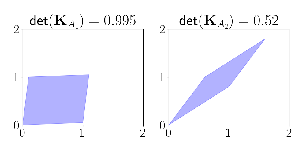
We see that the determinant for the uncorrelated set $A_1$ is larger, and the parallelogram is more “blocky.” On the other hand, the parallelogram for the correlated set $A_2$ is more elongated, leading to a smaller area and determinant.

$\mathbf{L}$-ensembles

Whereas the above definition considers the probability that subsets belong to $\mathcal{Y},$ we can also consider the probability over instantiations of $\mathcal{Y}$ itself. This yields an important special case of DPPs known as $\mathbf{L}$-ensembles, which are defined by a symmetric positive definite matrix $\mathbf{L}.$ For $\mathbf{L}$-ensembles, we have

where $\mathbf{L}_Y$ is the submatrix of $\mathbf{L}$ corresponding to the elements of $Y.$ This special type of DPP is especially useful in statistics and machine learning, where many data models already depend on a symmetric positive definite matrix. In different settings, this may be referred to as a kernel matrix, correlation matrix, or covariance matrix.

Sampling

Since a DPP is a distribution over sets, we can sample from this distribution. One of the first and most straightforward algorithms for sampling was introduced by Hough et al. in 2006. We review their algorithm here.

Given eigenvectors $\mathbf{v}_1, \dots, \mathbf{v}_n$ and eigenvalues $\lambda_1, \dots, \lambda_n,$ the algorithm proceeds in two stages. In the first stage, we sample a subset of the eigenvectors, which determines the size of the sample. In the second stage, we iteratively sample elements from these eigenvectors (one sample from each eigenvector).

An outline of the algorithm is below (adapted from Kulesza and Taskar), where $\mathbf{e}_i$ is the $i$th unit basis vector of length $n$.

1. $J \leftarrow \emptyset$
2. for $i = 1, \dots, n$: # Phase 1
   1. $J \leftarrow J \cup \{i\}$ with probability $\frac{\lambda_i}{\lambda_i + 1}$
3. $V \leftarrow \{\mathbf{v}_i\}_{i \in J}$
4. $Y \leftarrow \emptyset$
5. while $|V| > 0$ # Phase 2
   1. Select $i$ from $\Omega$ with probability $\frac{1}{|V|} \sum_{v \in V}(\mathbf{v}^\top \mathbf{e}_i)^2$
   2. $Y \leftarrow Y \cup i$
   3. $V \leftarrow V_{\perp},$ where $V_{\perp}$ is an orthonormal basis for the subspace of $V$ orthogonal to $\mathbf{e}_i$
6. Return $Y$

The algorithm forms a random subset $Y$ by sampling form each eigenvector. In step 5.3, we effectively condition on the fact that we just sampled element $i,$ which makes it less likely that we’ll sample elements similar to $i$ in subsequent iterations. This step can be performed with a Gram-Schmidt normalization procedure.

A Python implementation for sampling is below.

import numpy as np
from scipy.linalg import orth

def sample_dpp(K):

  eigvals, eigvecs = np.linalg.eigh(K)

  ### Phase 1 ###

  bernoulli_probs = eigvals / (eigvals + 1)
  bernoulli_trials = np.random.binomial(n=1, p=bernoulli_probs)
  J = np.where(bernoulli_trials == 1)[0]

  ### Phase 2 ###

  V = eigvecs[:, J]
  V_size = V.shape[1]
  Y_idx = np.zeros(len(J)).astype(int)

  for iternum in range(len(J)):

    # Randomly choose element
    probs = np.sum(V ** 2, axis=1)
    probs = probs / probs.sum()
    new_Y_idx = np.random.choice(np.arange(n), p=probs, replace=False)
    Y_idx[iternum] = new_Y_idx

    # Delete one eigenvector not orthogonal to new_Y_idx 
    # and find new basis
    j = (np.abs(V[new_Y_idx, :]) > 0).argmax()
    Vj = V[:, j]
    subspace = V - (np.outer(Vj, (V[new_Y_idx, :] / Vj[new_Y_idx])))

    V = orth(subspace)

  return Y_idx

One-dimensional example

Let’s consider a small example. Suppose our ground set $\Omega$ consists of $200$ scalar elements that are linearly spaced in $[0, 1].$ Let’s visualize how the sampling process works by showing the probability of sampling each element on each step of the second phase of the algorithm.

Below, the elements of $\Omega$ are represented on the $x$-axis, and the probability of sampling each element is shown on the $y$-axis. On each iteration, we plot the element that was sampled as a red bar on the bottom of the plot, and we update the probabilities over elements.

We can see that once an element is sampled, the probability of sampling similar elements (elements nearby) goes down. In the end, this yields a final set of samples that is diverse, and these elements can be thought of as “repelling” one another.

Two-dimensional example

We can also consider a setting in which $\Omega$ consists of two-dimensional elements. Let’s try an experiment where there are $900$ elements in $\Omega,$ with each one evenly spaced in the unit square. Below, we show a similar animation as the one above, but here each point represents an element of $\Omega,$ and we re-color the points on each iteration corresponding to their selection probailities.

References

• Hough, J. Ben, et al. “Determinantal processes and independence.” Probability surveys 3 (2006): 206-229.
• Kulesza, Alex, and Ben Taskar. “Determinantal point processes for machine learning.” arXiv preprint arXiv:1207.6083 (2012).